Center for High Angular Resolution Astronomy Center for High Angular Resolution Astronomy Center for High Angular Resolution Astronomy
                Center for High Angular Resolution Astronomy


CHARA

  • About
    • CHARA: An Overview
    • The CHARA Consortium
    • CHARA Facility and Instruments
    • Basics of Interferometry
    • CHARA Public Site
    • Mount Wilson Observatory
  • News
    • Science Press Releases
    • Announcements
  • Meetings
    • Annual Science Meetings
    • Community Workshops
  • Research
    • Journal Articles
    • Books and Review Articles
    • Technical Reports
    • Popular Press
    • CHARA Science
  • Observing
    • CHARA Facility and Instruments
    • Applying for Observing Time
    • Planning an Observation
    • Logistics of Observing
    • Observing Schedule
    • Remote Observing
    • Data Reduction Software
    • Data Analysis Software
    • Database
    • Acknowledgments
    • Weather
    • UCSD HPWREN Cameras
    • CHARA Wiki
  • Multimedia
    • Image Gallery
    • Photo Tour of CHARA
    • Videos
    • Mount Wilson and CHARA panorama
    • Drone Panoramas
  • Staff
    • CHARA Team
    • Contacts & CHARA directory

Overview of Reduction Steps

For MIRC-X 6T data obtained after the MIRC-X commissioning in June 2017, please use the MIRC-X python reduction pipeline and follow the instructions in the MIRC-X Pipeline User Manual.

The pipeline to reduce older MIRC data was written by John Monnier in IDL.  The pipeline and the archive of coadded MIRC data are available on the Remote Data Reduction Machine in Alanta. The source code is maintained at the University of Michigan through the Subversion control system.

There are three versions of the MIRC pipeline installed on the Remote Data Reduction Machine.  They are called using the following IDL startup scripts:

  • mirc6b_idl: Starts pipeline_mirc6b that reduces MIRC 6T data and accounts for cross-talk.
  • mirc6T_idl: Starts pipeline_mirc6 that reduces MIRC 6T data.  It does not account for cross-talk.
  • mirc4T_idl: Starts pipeline_v2 that reduces MIRC 4T data.

John Monnier has created an IDL mircx_cal.script routine to calibrate MIRC-X/MYSTIC data. The data would be processed using the standard mircx_reduce.py, but then mircx_cal.script could be used instead of mircx_calibrate.py. To use the IDL calibration routine enter the following startup script and follow the instructions for the calibration step described at the bottom of the page:

  • mircx_idl: Starts pipeline that can be used to calibrate mircx/mystic data. Note that mircx_reduce.py must be used before running mircx_cal.script. You will need to create mircx_aliasfile.txt and mircx_calibrators.txt before running mircx_cal.script (see descriptions below).

Below is a listing of the steps to run when reducing 6T or 4T MIRC data.  Each step is described in more detail in the sections below.

MIRC 6T Data (with photometric channels: 2011 July - 2017 May)

To reduce MIRC 6T data, use the mirc6b_idl or mirc6T_idl startup procedures.  The 6b version of the pipeline is recommended, especially for bright resolved targets, because it accounts for cross-talk between baselines.  The 6b version takes longer to run.

  • $ mirc6b_idl
  • IDL> mirclog, date='2011Sep29', coadd_path='/dbstorage/mircs/MIRC_COADDp/', /verbose
  • IDL> .r mirc_process2.script
  • IDL> .r mirc_process3.script
  • IDL> .r mirc_process4.script
  • IDL> .r mirc_process5.script
  • IDL> .r mirc_average_sigclip.script  ---OR--- IDL> .r mirc_average.script
  • IDL> .r mirc_cal.script

MIRC 4T Data (No photometric channels: 2006 June - 2009Aug; With photometric channels: 2009Aug23 - 2011Jan19)

To reduce MIRC 4T data, use the mirc4T_idl startup procedure.

  • $ mirc4T_idl
  • IDL> mirclog, date='2010Nov05', coadd_path='/dbstorage/mircs/MIRC_COADDp/', /verbose
  • IDL> .r mirc_process2.script
  • If NO XCHANS then run IDL> .r mirc_process3.script
  • If XCHANS then run IDL> .r mirc_process3xchan.script
  • IDL> .r mirc_process4.script
  • IDL> .r mirc_process5.script
  • IDL> exit
  • The last two steps need be run using the pipeline_mirc6 (not 6b) startup file:
  • $ mirc6T_idl
  • IDL> .r mirc_average_sigclip.script  ---OR--- IDL> .r mirc_average.script
  • IDL> .r mirc_cal.script

Additional Files Needed to Reduce MIRC 4T data:

  • For data prior to UT 2009Aug23 without photometric channels, the photometry for each beam was monitored by spinning chopper blades at different frequencies in front of each beam.  For some of these dates, synchronization of the choppers were time tagged by DAQ synchronization.  The DAQ synchronization files are not yet in the Atlanta archives, so check with John Monnier to see if the DAQ files exist in the Michigan archives.  If these files exist, the DAQ sync data path is identified by a DAQDIR line added to the mirclog file.
  • When running mirc process 3, the pipeline will query the user for a comboinfo.idlvar file.  For H-PRISM data obtained with MIRC, please download the linked template comboinfo file to load as an initial guess for the wavelength solution.  The pipeline then solves for the wavelength solution more precisely for the given night.  After downloading the template, rename the file using the appropriate UT date for the data that is being reduced and place it in the working directory. That way the pipeline will overwrite the old file with the updated solution.

Locating the Coadded MIRC Data

Coadded MIRC data are available on the Remote Data Reduction Machine in Atlanta in the following location:

/dbstorage/mircs/MIRC_COADDp

These data have been already run through mirc_process1.script which does the following steps:

  1. Remove unused quadrants (keeps two quadrants for fringe data and photometric channels).
  2. Coadd nreads.
  3. Sigma filter the difference frames, but restack so the data look like raw data.
  4. Look for data dropouts and add keyword BADFLAG to header (=0 for OK or 1 for bad).
  5. Output files to MIRC_COADD directory.
  6. Add line to header regarding saturation estimate.

For data obtained between UT 2013 Apr 19 and 2013 Aug 01, use coadded data processed using mirc_process1rf.script which suppresses RF noise by subtracting signal from the neighboring quadrant.  These coadded data can be found in the following location:

dbstorage/mircs/MIRC_COADDrf

Starting the MIRC IDL Pipeline

Create a working directory on the Remote Data Reduction Machine.  Change directories to the working directory and start the MIRC IDL pipeline using the appropriate startup script (mirc6b_idl, mirc6T_idl, mirc4T_idl):

$ mirc6b_idl

Create MIRC Log File

Run mirclog.pro to create the .mirclog file:

IDL> mirclog, date='2011Sep29', coadd_path='/dbstorage/mircs/MIRC_COADDp/', /verbose

The .mirclog groups each target into DATA sequences and SHUTTER sequences (BG = Background; B1-B6 = single beam shutters; FG = foregrounds, light from all telescopes but no fringes).

Edit the .mirclog file by comparing to the hand-written observing logs.  Copies of the scanned observing logs are available in the shared MIRC google drive.  Check to make sure the beam order is correct and that the correct shutter blocks are identified for each data block.  The associated shutter block is identified in the last column of each DATA line.  The #Fiber Explorer notes are sometimes located at the wrong positions in the .mirclog file, so it is important to make sure that the DATA and SHUTTER sequences are identified correctly, particularly when repeated data sets are obtained on the same target.  Remove any files where a beam was lost during the shutter sequences.  If possible, there should not be a fiber explorer map between the data and the associated shutters.

Prior to the installation of the photometric channels (in August 2009), in addition to the DIR line for the data directory, the mirclog file should also contain a line for the DAQDIR which contains the directory path for the DAQ synchronization files for synchronized chopping.

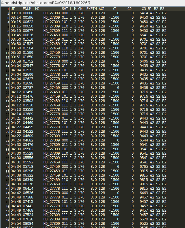
 Here is an example of an edited MIRC log file:

$ more 2011Sep29.mirclog
## MIRC Log for 2011Sep29
## Automatically created by mirclog.pro on Wed Jun 24 15:29:34 2020
## Hand-Edited by ___GHS___ on ___2020Jul06___
##
DIR   /dbstorage/mircs/MIRC_COADDp/2011Sep29/
##Source             MODE     Block  Type  Start  End    SHUTBLOCKS
## Include only one BEAM ORDER per MIRCLOG FILE !!!
BEAM_ORDER W1 S2 S1 E1 E2 W2 
## Fiber Explorer
HD_25490             H_PRISM  12     DATA  1274   1333   13
HD_25490             H_PRISM  13       BG  1334   1343
HD_25490             H_PRISM  13       B1  1344   1353
HD_25490             H_PRISM  13       B2  1354   1363
HD_25490             H_PRISM  13       B3  1364   1373
HD_25490             H_PRISM  13       B4  1374   1383
HD_25490             H_PRISM  13       B5  1384   1393
HD_25490             H_PRISM  13       B6  1394   1403
HD_25490             H_PRISM  13       FG  1404   1413
##
## Fiber Explorer
HD_33256             H_PRISM  14     DATA  1414   1473   15
HD_33256             H_PRISM  15       BG  1474   1483
HD_33256             H_PRISM  15       B1  1484   1493
HD_33256             H_PRISM  15       B2  1494   1503
HD_33256             H_PRISM  15       B3  1504   1513
HD_33256             H_PRISM  15       B4  1514   1523
HD_33256             H_PRISM  15       B5  1524   1533
HD_33256             H_PRISM  15       B6  1534   1543
HD_33256             H_PRISM  15       FG  1544   1553
##
## Fiber Explorer
HD_37468             H_PRISM  16     DATA  1554   1613   17
HD_37468             H_PRISM  17       BG  1614   1623
HD_37468             H_PRISM  17       B1  1624   1633
HD_37468             H_PRISM  17       B2  1634   1643
HD_37468             H_PRISM  17       B3  1644   1653
HD_37468             H_PRISM  17       B4  1654   1663
HD_37468             H_PRISM  17       B5  1664   1673
HD_37468             H_PRISM  17       B6  1674   1683
HD_37468             H_PRISM  17       FG  1684   1703
##
## Fiber Explorer
HD_33256             H_PRISM  18     DATA  1704   1763   19
HD_33256             H_PRISM  19       BG  1764   1773
HD_33256             H_PRISM  19       B1  1774   1783
HD_33256             H_PRISM  19       B2  1784   1793
HD_33256             H_PRISM  19       B3  1794   1803
HD_33256             H_PRISM  19       B4  1804   1813
HD_33256             H_PRISM  19       B5  1814   1823
HD_33256             H_PRISM  19       B6  1824   1833
HD_33256             H_PRISM  19       FG  1834   1853
##
## Fiber Explorer
HD_37468             H_PRISM  20     DATA  1854   1913   21
HD_37468             H_PRISM  21       BG  1914   1923
HD_37468             H_PRISM  21       B1  1924   1933
HD_37468             H_PRISM  21       B2  1934   1943
HD_37468             H_PRISM  21       B3  1944   1953
HD_37468             H_PRISM  21       B4  1954   1963
HD_37468             H_PRISM  21       B5  1964   1973
HD_37468             H_PRISM  21       B6  1974   1983
HD_37468             H_PRISM  21       FG  1984   2003

Note: Data obtained earlier on this night was collected in K-band mode.  Those data were edited out of the .mirclog file to process only the H_PRISM data.

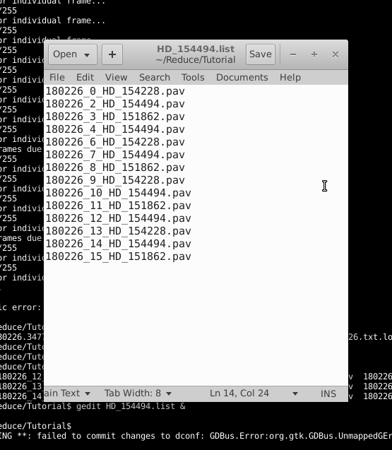
Create Alias and Calibrator Files

The MIRC IDL pipeline uses the file mirc_aliasfile.txt to identify the preferred name of each target observed and mirc_calibrators.txt to specify the calibrator diameters.  The format of each of these files are shown below.  If a target does not appear in either of these files, then the pipeline will query the user for the necessary information.

$ more mirc_aliasfile.txt 
Alternative ID, MIRC ALIAS
* nu. Tau,HD 25490
HD 25490,HD 25490
* 68 Eri,HD 33256
HD 33256,HD 33256
* sig Ori,sig Ori
sig Ori,sig Ori

NOTE: Create a mirc_aliasfile.txt in your working directory containing at least the first header line "Alternative ID, MIRC ALIAS". If this file does not exist, then the mirc_process2.script will crash.

$ more mirc_calibrators.txt
HD_25490   0.599   0.020   SED_Fit_HD25490
nu_tau     0.599   0.020   SED_Fit_HD25490_nuTau
HD_33256   0.655   0.018   SED_Fit_HD33256

To reduce MIRC 4T data, you also need to create a .mircarray file that specifies which telescope is on which beam and an initial comboinfo.idlvar file.  For the comboinfo file, you can download the sample idlvar file available in the link above and change the file name to the correct date. An example mircarray file for the S1E1W1W2 configuration is shown below (change the telescope configuration as needed):

$ more 2010Nov_S1E1W1W2.mircarray
## Enter Array Information  NEED TO CHECK AND EDIT, NOT SURE WHETHER IT IS THE RIGHT INFO!!!
MIRC    4
B1      S1
B2      E1
B3      W1
B4      W2

Calculate uv coverage and time information

The routine mirc_process2.script calculates the uv coverage and time information.  It creates a YYYYMMMDD.idlvar file that is used during the few next steps of the pipeline. 

IDL> .r mirc_process2.script

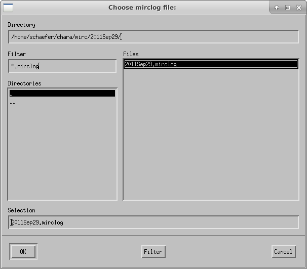
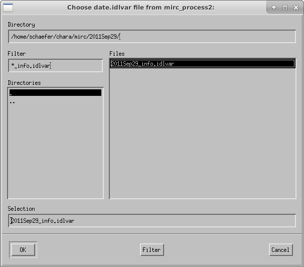
The script will ask the user to select the mirclog file:

Choose mirclog file.


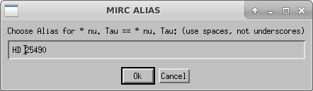
If a target is not already in mirc_aliasfile.txt, the script will ask the user to choose an alias for each target. Remember that you need to create a file called mirc_alias.txt in your working directory that contains, at minimum, the header line "Alternative ID, MIRC ALIAS".  If the mirc_alias.txt file does not exist, then the pipeline will crash.

Choose alias.


Compute Photometry

The next step is to run mirc_process3.script to compute photometry information.

IDL> .r mirc_process3.script 
Interactive (1,default) or automatic (0):

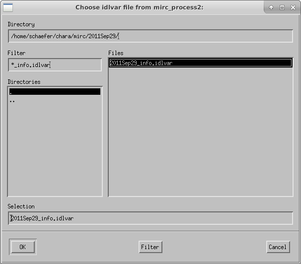
The script will ask the user to select the idlvar file created during mirc_process2:

Choose idlvar file.


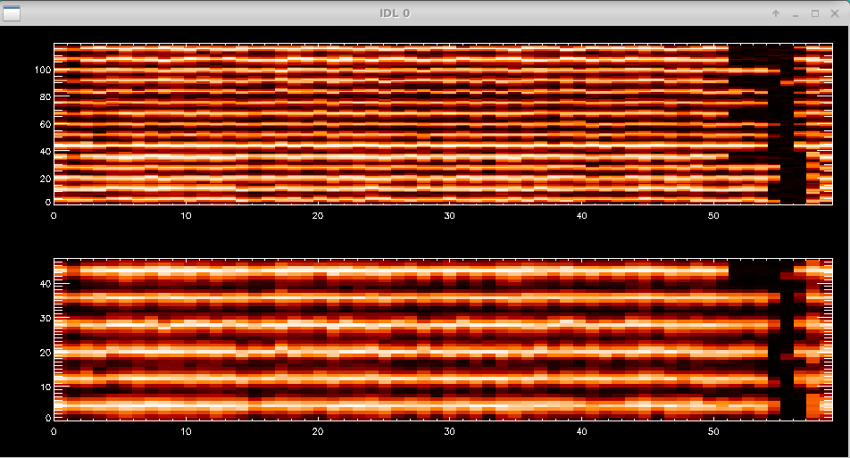
The script then displays the profiles for data and xchan regions of the detector during the data and shutter sequences:

Profiles for data and shutter sequences.


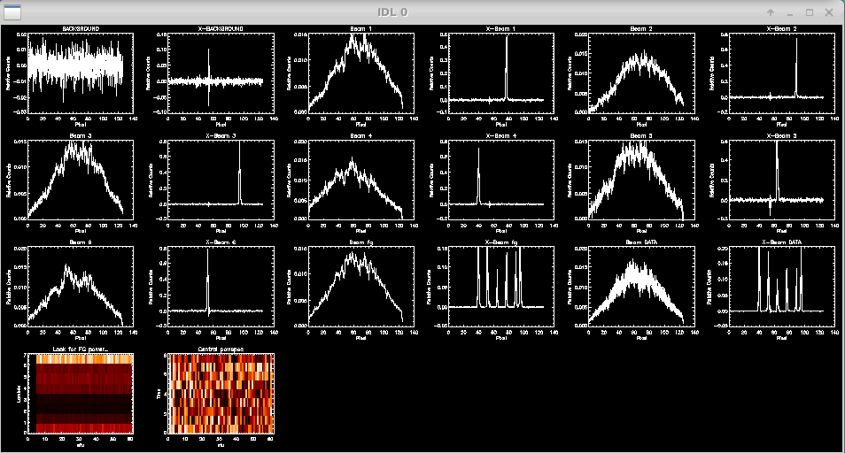
Check to see if light is on all of the beams and to make sure there are no fringes in the foreground frames. The script will prompt the user to flag missing beams or identify bad foreground frames. If all is good, then hit enter to continue.

OK? hit enter to continue
hit n to remove FG files due to fringes in the FG
hit numbers 1,2,3,4,5,6 to mark one beam as missing
HD_25490      12
: 

Next the script will plot the flux over time for each beam as measured from the photometric channels (xchan). The vertical dashed lines separate the data, shutter, and foreground files. The beam ratios are printed to the screen.

Photometry in each beam.


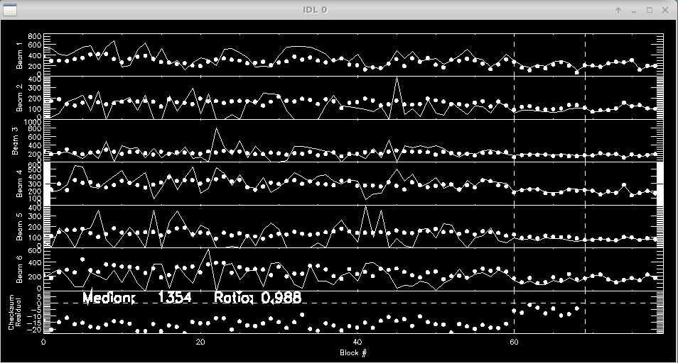
 Ratio Check: 
Channel: 00   Ratio: 0.986 +/- 0.001
Channel: 01   Ratio: 0.987 +/- 0.001
Channel: 02   Ratio: 0.985 +/- 0.001
Channel: 03   Ratio: 0.989 +/- 0.001
Channel: 04   Ratio: 0.991 +/- 0.001
Channel: 05   Ratio: 0.992 +/- 0.001
Channel: 06   Ratio: 0.992 +/- 0.001
Channel: 07   Ratio: 0.983 +/- 0.001
 End of block loop. hit enter to continue
: 

The script will loop through these profile and flux plots for each target.

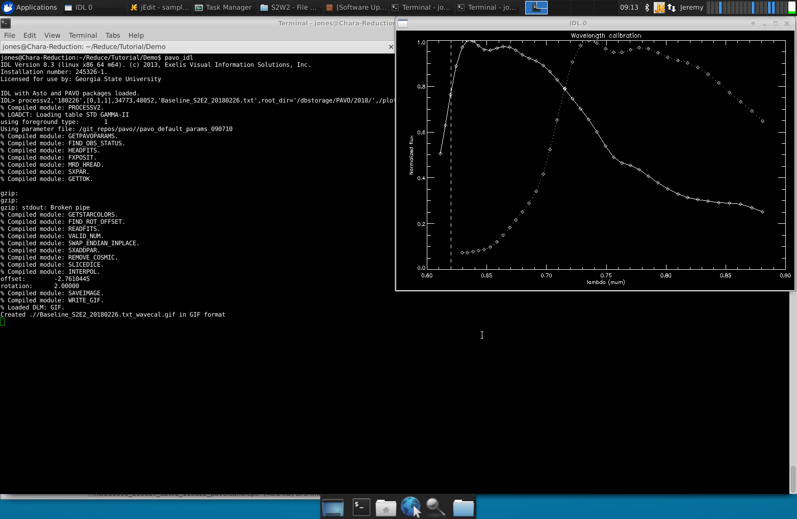
Optimize fringe information for  given combiner setup

Run mirc_process4.script to optimize fringe information for a given combiner setup.  This step produces the date_comboinfo.ps file.

IDL> .r mirc_process4.script

The script will ask the user to select the idlvar file and will continue on from there:

Choose idlvar file.


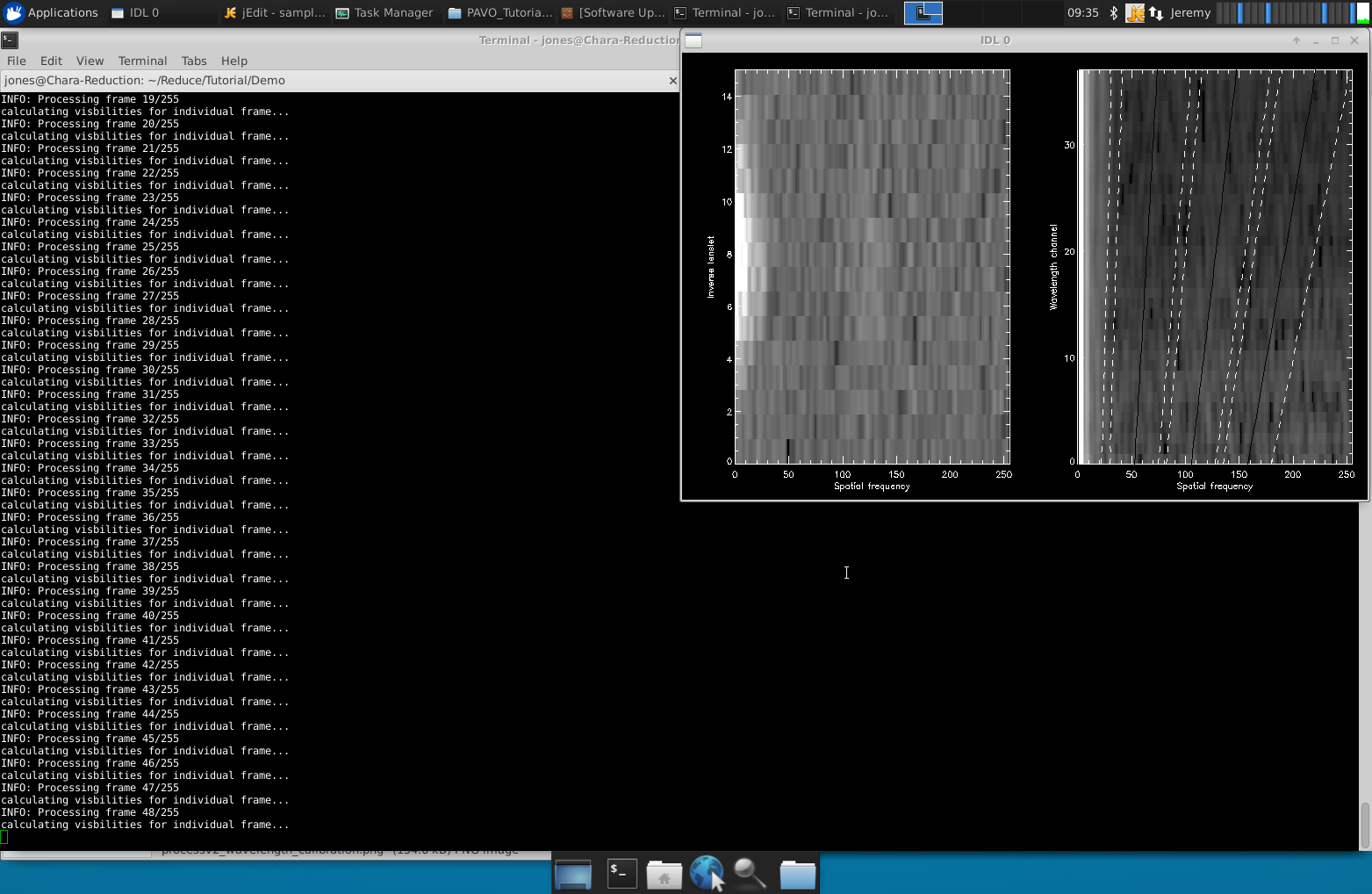
Coherent Integration

Run mirc_process5.script to compute coherent integration.  It is recommended to run this step twice, once with the default integration time of 17 ms and another time with a longer coherent integration time of 75 ms.  The longer coherent integration time will improve signal-to-noise for faint targets.  However, the shorter integration time might be necessary in bad seeing conditions to avoid biasing the visibility calibration.  A comparison of the results between the two coherent integration times can help decide the optimal value. This step creates the date_tcoh0017ms_diagnostics.ps summary file.

IDL> .r mirc_process5.script
Enter coherent integration time
 (default: 17 ms; for faintest targets try 75 ms)
: 17 

The script will ask the user to select the idlvar file:

Choose idlvar file.


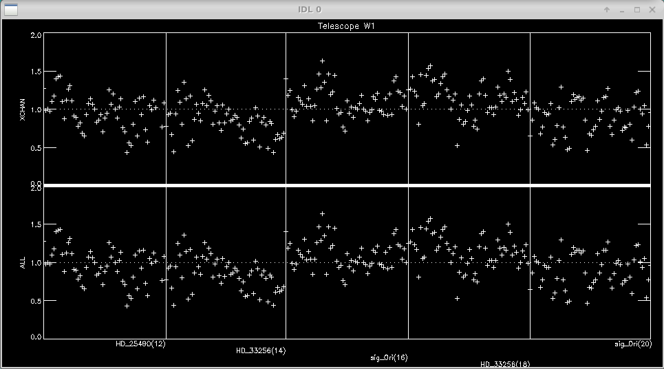
The script will then show the waterfall fringe plots for each target.  The top panel shows the fringes for each baseline separately.  The lower panel shows fringes summed over all pairs for each telescope.  Dropouts from a particular telescope can be identified more easily in the bottom panel.

Plots of fringe waterfall displays.


Data Editing and Averaging

Run mirc_average.script or mirc_average_sigclip.script to average data and remove bad data points.  Both scripts allow the user to interactively remove bad data points.  The sigclip version applies sigma clipping to automatically remove data points that are more than 3 standard deviations discrepant from the median.  After sigma clipping, the user can still interactively reject additional data points.  The sigma clipping option provides a less subjective way to remove discrepant data points.  If you want to run a quick reduction without scrolling through all of the sigma clipping plots, then use mirc_average.script instead.

The data are averaged over a default time interval of 2.5 min.  The routine will save raw level one MIRC_L1*.oifits and summary MIRC_LI*.ps files for each target in the OIFITS output directory. 

IDL> .r mirc_average_sigclip.script

--- or ---

IDL> .r mirc_average.script

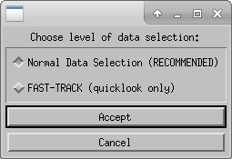
Choose the level of data selection (Normal Data Selection is recommended):


Choose the idlvar file:


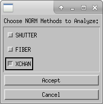
Choose normalization method to analyze.  XCHAN is preferred, but can be compared to other flux methods if necessary:


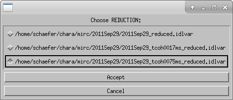
Choose which reduction to process (e.g., 17 ms or 75 ms coherent integration time from the previous step):


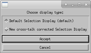
Choose display type (default):


Select the Maximum Averaging time (2.5 min is the default):


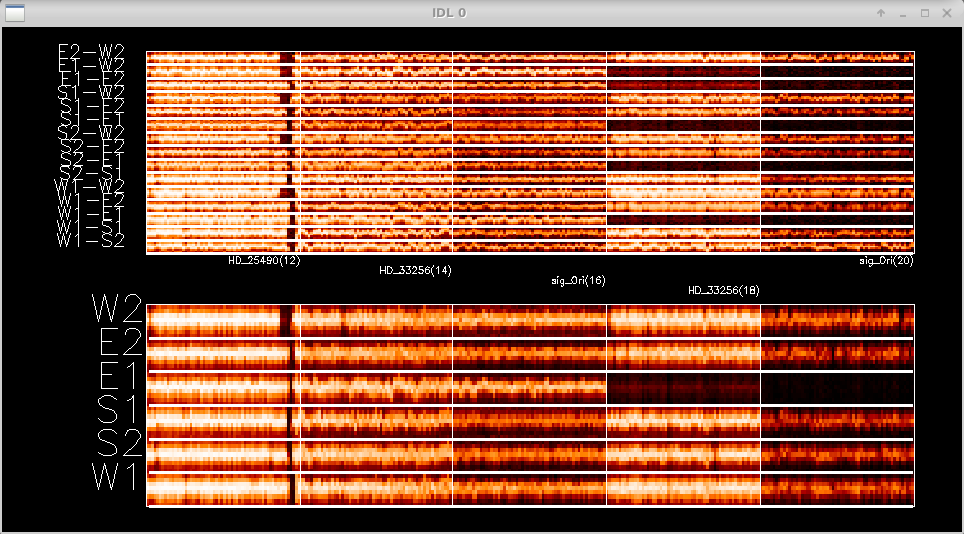
Next you can edit data based on the fringe waterfall plots.  The top panel shows the fringes for each baseline separately.  The lower panel shows fringes summed over all pairs for each telescope.  Dropouts from a particular telescope can be identified more easily in the bottom panel.  The target name is written for each panel.  Follow the instructions on the terminal window to edit fringes.

Fringe editing.


 Double click in a square to flag whole block as bad (<0.5 sec)
 Click twice over a range to flag a specific RANGE 
 Click to the right of plot to REPLOT (allows to resize window)
 Click below all plots to reset bad flags!!
 Click to the left of plots to continue.. 

Next you can edit data based on the flux from each telescope.  The pipeline loops through the flux rejection for each telescope.  Follow the instructions on the terminal window to edit any dropouts in flux.

Flux editing.


 Double click in a square to flag whole block as bad (<0.5 sec)
 Click once to mark a single point as bad
 Click to the right of plot to REPLOT (allows to resize window)
 Click below all plots to reset bad flags!!
 Click to the left of plots to continue.. 

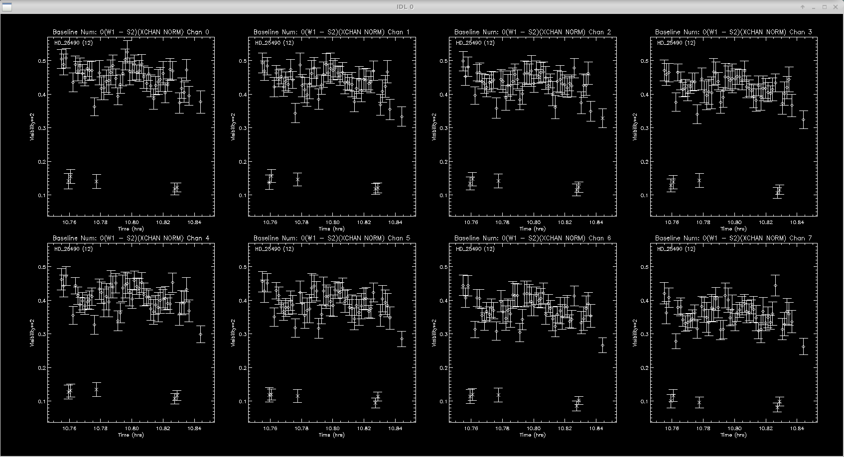
Next the script will ask if you want to apply sigma clipping to the visibilities.  It will loop through each baseline and show a plot for each target.  The panels show the data in each of the 8 spectral channels.  Follow the instructions on the screen to change the sigma clipping parameters and press enter to reject the clipped measurements after each plot.

Would you like to apply sigma clipping?
(applies to visibilities, closure phases, and closure amplitudes)
<Y>  or N
: Y
Sigma clipping rejection threshold (N*stdev): 
      3.00000
Would you like to change rejection threshold?
Y of <N>
: N
------------------------------
Sigma clipping of visibilities
Rejection threshold (N*sigma):       3.00000
NOTE: Edge channels will not be used to apply sigma clipping flags
Hit enter to continue
: 
Block:       12  Source: HD_25490
Diamonds - good data; X - sigma clipped
Number of measurements on target (per spectral channel): 
          57
Maximum number of sigma clipped measurements per spectral channel: 
      7.00000
Number of uniquely rejected measurements (not including edge channels): 
       7
Do you want to reject these measurements?
<Y> or N:
: 


Sigma clipping.  The diamonds are good data and the x's are rejected data.


 Calculating Calibration Table for All Spectral Channels...
----------------------------------------
Finished sigma clipping the visibilities.
Begin visual inspection and flagging of visibilities.
Hit enter to continue
: 

The next step is the interactive data editing.  The script will loop through each baseline and show all targets in only one spectral channel.  The sigma clipping routine will remove most of the outliers, but its good to double check and edit where needed.  Follow instructions on screen to remove data points.

Interactive Visibility Rejection


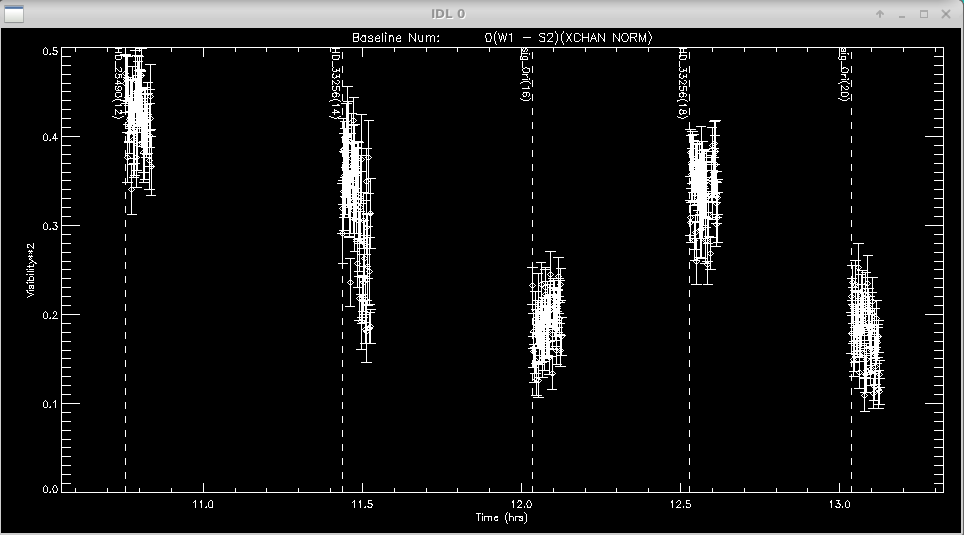
 Click left of axis to continue (or to goback to unzoomed view)
 Click right of axis to change smoothing length
 Click near datapoint to remove a time sample.
 Click below axis twice to specify a range to remove.
 Click above plot twice to specify a range to ZOOM up

The same procedure of sigma clipping and interactive editing is then repeated for the closure phases and triple amplitudes on all closure triangles.

Data Calibration

The last step runs mirc_cal.script to calibrate the science data using the calibrator observations and estimated calibrator diameters.

IDL> .r mirc_cal.script

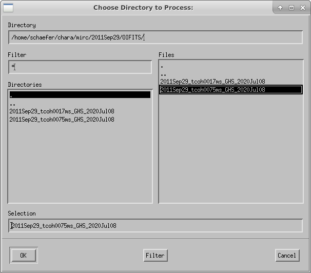
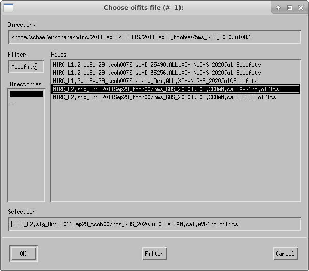
The script will ask the user to choose the directory to process:


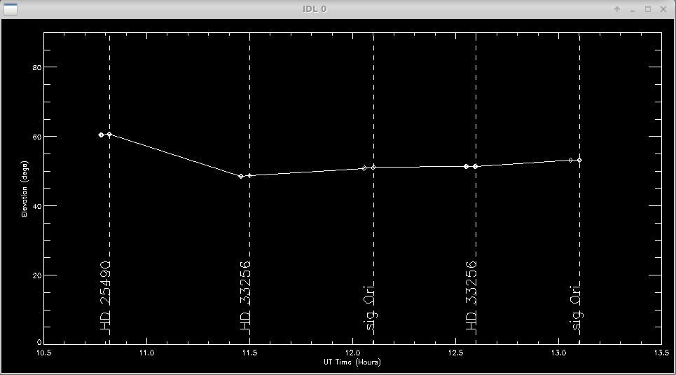
A plot of the target elevation vs time is shown:

Plot of target elevation vs. time.


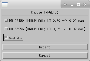
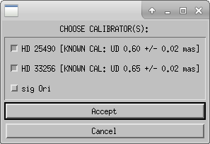
Next the user will select science targets and then calibrator stars from the list of stars observed during the night.  The user can choose to process science targets and calibrators located in the same region of the sky by selecting only those stars from the list.


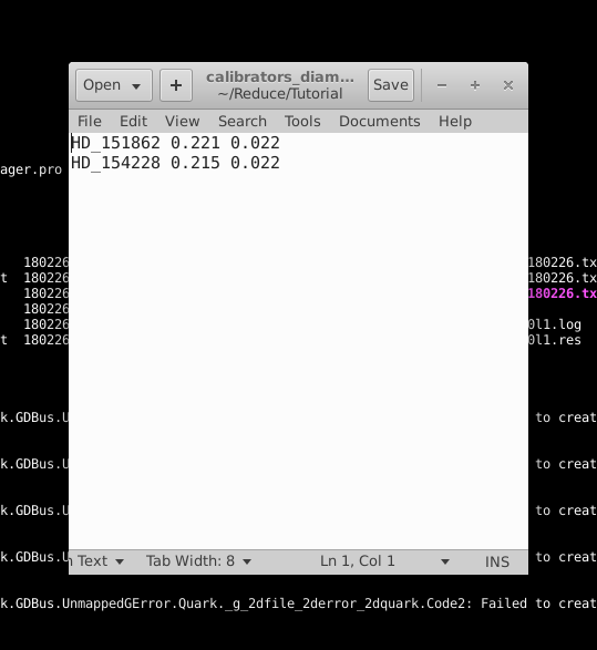
The routine will search the mirc_calibrator.txt file to find the calibrator diameters.  If a calibrator is not included in the file the routine will query the user for the diameter.  After the diameters are read from the file, the user will confirm the adopted diameters in the terminal window.

 
 CALIBRATOR DIAMETER FOUND: 
 target  udsize (mas), err: HD 25490     0.599000    0.0200000 (SED_Fit_HD25490)
 Would you rather use an alternative calibration model?
Y or <N> :  
 CALIBRATOR DIAMETER FOUND: 
 target  udsize (mas), err: HD 33256     0.655000    0.0180000 (SED_Fit_HD33256)
 Would you rather use an alternative calibration model?
Y or <N> : 

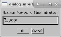
Next the user will choose the maximum averaging time for an observing block (default is 15 min).  The user might consider increasing the maximum averaging time if a single set of observations on a target took longer than 15 min.  The length of an observing block is typically between 10-30 minutes.


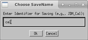
Enter the file extension for saving the calibrated oifits files. If you need to re-run the calibration, you can change the extension to avoid copying over existing files.


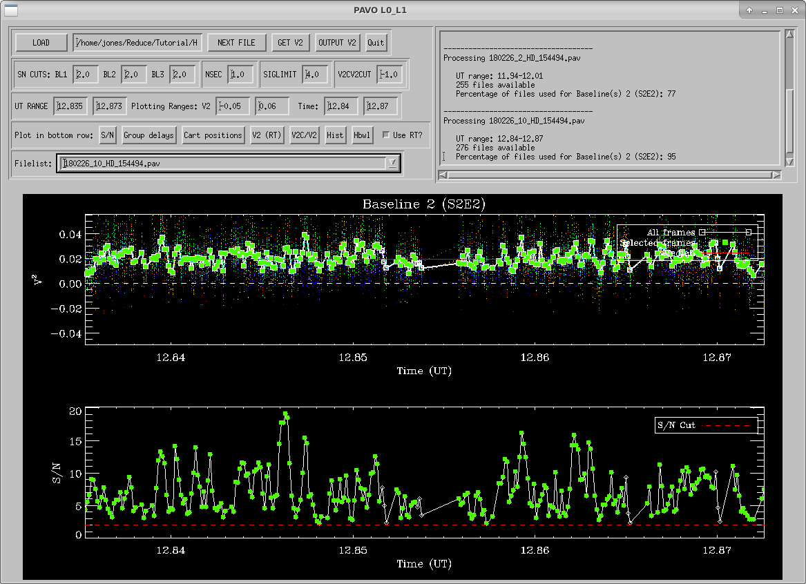
The program will make plots of the calibrator and target visibilities vs. time for each baseline.  The transfer function is overplotted.  The options printed to the terminal window allow the user to cycle through the wavelength channels and to flag bad data points.

Visibility vs. time for calibrators and science targets.


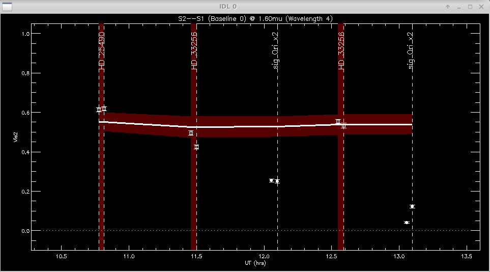
 Click left of axis to continue to next baseline
 Click near point to remove it (be careful: there is no UNDO)
 Click above graph to cycle through wavelengths
 Click to the right to change the xfer function parameters (timescale, sky_scale)
 Click time range below axis to see an alternative view of 
     multi-wavelength calibrated vis2 for data selection / bad flagging convenience

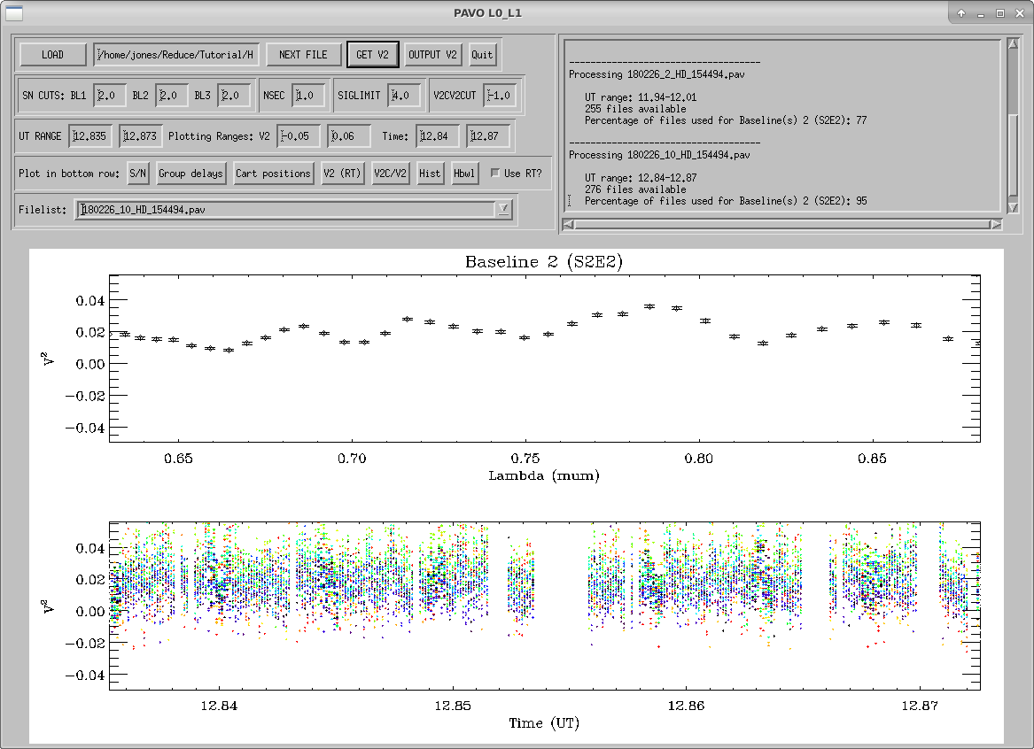
It is useful to zoom in on a particular target or calibrator to view the visibilities over all wavelength channels. The first and last wavelength channels sometimes show low signal-to-noise, particularly for faint targets, and might need to be removed.

Zoomed in visibility plot showing all spectral channels for the selected target.


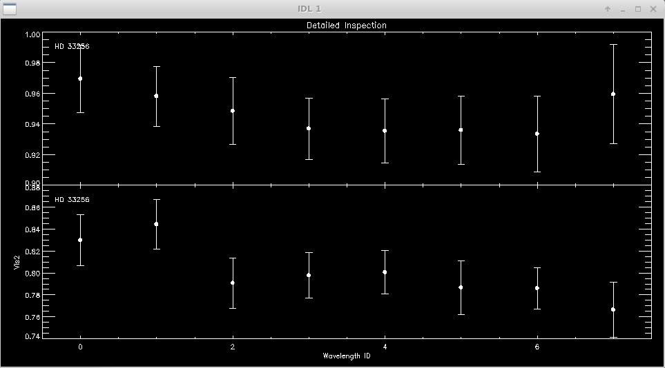
Click next point: 
WINDOW 1 OPTIONS:
  Click near point to remove it (be careful: no UNDO)
  Click left of axis to return
  Click below axis to mark ALL POINTS AS BAD (NUCLEAR OPTION)

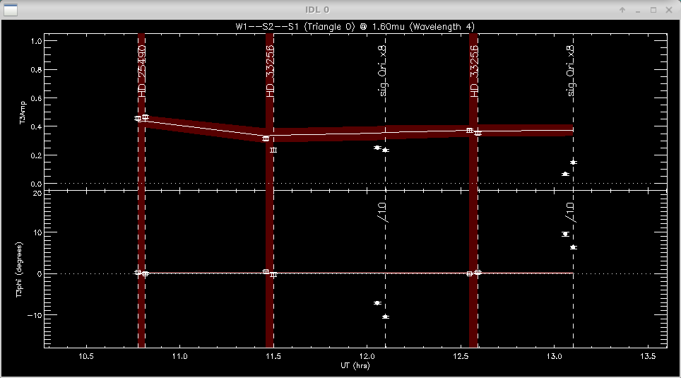
The same process is repeated for the closure phases (T3phi) and triple amplitudes (T3amp) for each closure triangle.

Triple amplitudes and phases vs. time.


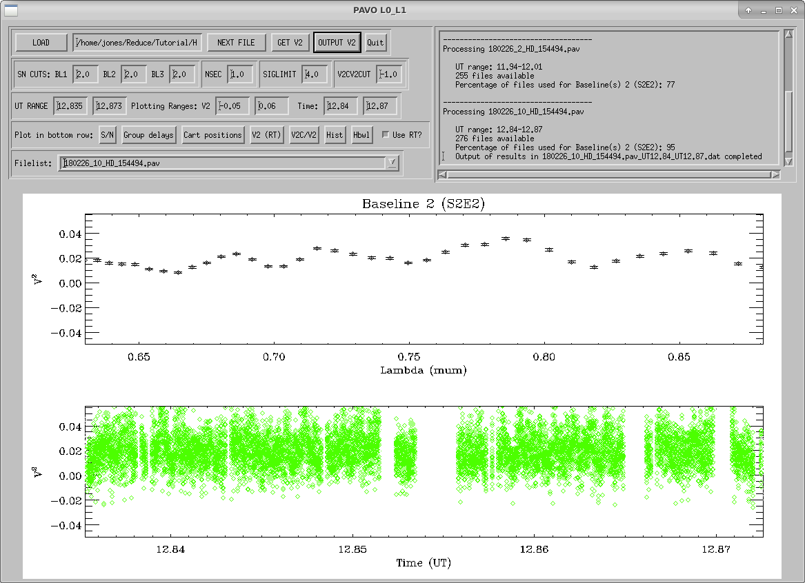
When completed, mirc_cal.script will save calibrated MIRC_L2*oifits and summary MIRC_L2*ps files for each science target in the selected OIFITS directory. For each target, the program produces two calibrated OIFITS files: the AVG15m.oifits are averaged over the 15 min observing blocks set in mirc_cal.script and SPLIT.oifits splits each observing block into 2.5 minute chunks of time defined by the averaging time set in mirc_average.script.  The summary ps files contain plots of the uv coverage, vis2 vs baseline, vis2 vs wavelength for each baseline, CP vs wavelength, and T3amp vs wavelength for each closure triangle.  The script also produces a file called XFER.XCHAN.cal_*.ps that plots the transfer fucntion for each baseline and closure triangle during the night.

Applying Standard MIRC Calibration Errors

After the reduction process is complete, run oifits_prep.pro to apply the standard MIRC calibration errors to the visibilities, closure phases, and triple amplitudes.  The file created during this step should be used in subsequent analysis.

IDL> oifits_prep

The program will ask the user to select the calibrated oifits file.  Multiple files can be selected if you want to merge separate observing blocks on the same target.  Hit OK to add another file or Cancel to continue.


Recommended calibration errors for 6T and 4T data are listed below:

Vis2 Error multiplier: 1.5 (default, use 1 to apply uniformly to all measurements)
Min Vis2 Additive Error: 0.001 (default)
Min Vis2 RELATIVE Error: 0.05 (use 0.05 default for MIRC-6T, use 0.10 for MIRC-4T no xchan)
t3amp Error multiplier: 1.5 (defaut, use 1 to apply uniformly to all measurements)
Min T3AMP Additive Error: 0.0002 (default)
Min T3AMP RELATIVE Error: 0.10 (default)
Min T3PHI ADDITIVE Error (degs): 0.30 (default)

The user then enters the output file name.


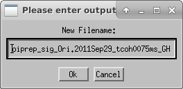
The file created during this step can then be used in subsequent analysis. 

The reduction process is finished!  Good luck with the model fitting, imaging, and analysis!


Adaptive Optics (AO) implementation is underway at the CHARA Array.  Beginning in the 2020A semester, all science operations will be conducted using the AO systems.  The CHARA adaptive optics program involves two separate AO systems: (1) a deformable mirror and wavefront sensor located at each telescope to provide tiptilt control and fast AO correction to compensate for atmospheric distortions, (2) a deformable mirror and wavefront sensor on each of the beam-reducing tables inside the lab to provide a slow AO correction for non-common path errors in beam transport from the telescope to the delay lines inside the lab.

All wavefront sensors are currently installed in the lab and the telescopes.  Small deformable mirrors are installed in the lab for all beams. Deformable mirrors are installed on all telescopes except for E2 and W2.  Currently, the telescope tiptilt and labAO loops are locked for all telescopes during observations.  The telescope AO loops are locked for S1, S2, E1, and W1.  We expect the deformable mirrors for E2 and W2 to be repaired and installed at the telescopes in the near future.

There are three beam splitters that can be used.  Each splitter sends a different percentage of visible light to the telescope AO system and into the lab.  The choice of AO beam splitter usually depends on the operating wavelength of the beam combiner:

  • IR AO beam splitter: sends more of the visible light to the telescope AO system.  The IR splitter is the standard for infrared combiners (CLASSIC, CLIMB, MIRC-X).
  • VIS AO beam splitter: sends more of the visible light to the lab.  The VIS splitter is the standard for visible light combiners (PAVO, VEGA).
  • BARE uncoated AO beam splitter: used for engineering purposes or for special target considerations.

The AO Beam Splitters Technical Report describes the splitters in more detail. Please consult with the CHARA staff if you have any questions on whether a non-standard AO beam splitter could be useful for your target priorities.


References:

The CHARA Array Adaptive Optics Program
ten Brummelaar et al., 2019 SPIE 107034

 The AO Beam Splitters at the Telescopes
J. Sturmann, 2020, CHARA Technical Report 101

PAVO Data Reduction Pipeline

The PAVO Data Reduction Software is available through the CHARA Git repository, but it is recommended that you use the already-installed copy of the software on the Remote Data Reduction Machine based on the CHARA Server in Atlanta. The tutorial below will assume you are using the Remote Data Reduction Machine. If you do wish to download the software and use it on your own system, you can do so by running the command git clone https://gitlab.chara.gsu.edu/fabien/pavo.git and you can update this software by running the command git pull in the directory created by the git clone command. You will also need the IDL astronomy library (astrolib), which can be found here. For more information on the math and physics behind the data reduction process, see the PAVO instrument paper (pdf here).

Locating your data

CHARA Data are organized in the archive by beam combiner, then date. For example, all raw PAVO data for UT night 2018 Feb 26 is in the directory /dbstorage/PAVO/2018/180226. If you do not know on what nights a target was observed, run the script find_pavo_target HD_number. This will read through the headstrip files (see below) and find on what nights the target was observed.

Using the find_pavo_target script.

It is important that the HD number for the star be in the format HD_XXXXX, because the find_pavo_target script looks for the target in the same format as it appears in the headstrip file.

Setting up the PAVO environment

The PAVO data reduction software is written in IDL. The command pavo_idl will start IDL and load the astrolib IDL library and the PAVO software library. When you start IDL in this manner, you should see the following startup message:

PAVO IDL startup

The headstrip.txt file

The first part of the data reduction process is to run the headstrip.pro program for the night of data you wish to reduce. We have already done this for all PAVO data currently in the archive, and we do this regularly as new PAVO data are copied to the archive. This program reads the header for each data file in the directory and outputs a text file in the data directory (headstrip.txt) containing the following information:

  • UT – UT time of the first file
  • FNUM – Starting file number
  • HD – HD number of the Target
  • SHT – Shutter status for beams B1, B2, and B3. “0” means open. “1” means closed. Taken as a whole, the three numbers indicate what part of the shutter sequence the data represent.
  • GN – Gain setting of the detector
  • EXPTM – Exposure time of the detector.
  • C1, C2, C3 – Offsets for the OPLE carts. The carts are moved away from the fringe position during the shutters, so you should expect a different value in the shutter sequence compared to the data sequence.
  • B1, B2, B3 – Identifies which telescope is on which beam

If you notice any discrepancies between your observing logs and the headstrip file, please discuss them with CHARA Data Scientist, Jeremy Jones before proceeding with your reduction as the headers on the data may need to be modified.

An example of the headstrip.txt file.

Tutorial Example - HD 154494

For this tutorial, we will reduce the data for one target and its two calibrators. These data were taken on UT 2018 Feb 26 with the S2-E2 baseline under decent seeing conditions (10.6 cm mean seeing for the night). Six observations were taken of the target, HD 154494, which is a V=4.8 magnitude star of type A3V with an estimated diameter of 0.38 mas (JMMC Stellar Diameter Catalogue). Four observations were taken of each calibrator. Both calibrators, HD 151862 and HD 154228, have V-band magnitudes of 5.9 mag and are A1V-type stars with estimated diameters of 0.22 mas.

Running processv2.pro

The first step of the reduction process that you will be running is processv2.pro. It can take several hours to run, so be prepared to wait. Processv2 requires the following to be set:

  • Data directory – The name of the directory the data are in (not the full path). E.g., 180226
  • The beams used – A vector of three integers of value 0 or 1 each representing which beams were used. E.g., [0,1,1] means beams 2 and 3 were used and [1,1,1] means all three beams were used.
  • Starting file number – The number of the first file to be reduced. If you are reducing an entire night, this will be 00000 but you should consult the headstrip.txt file for your data if you are only reducing a portion of the night or if different configurations were used during the night.
  • Ending file number – The number of the last file to be reduced.
  • Output filename – The name you wish to give to the output file
  • Root directory – The directory that the data directory is

In our example, we will call the processv2 command like this:

processv2,’180226’,[0,1,1],34773,48052,’Baseline_S2E2_20180226.txt’,root_dir=’/dbstorage/PAVO/2018/’,/plot,/individual

In this case, 180226 is the data directory, [0,1,1] indicates we were using beams 2 and 3, 34773 is our starting file number, 48052 is our ending file number, Baseline_S2E2_20180226.txt is the name we’ve given to the output file, /dbstorage/PAVO/2018/ is the full path to the data directory, and the /plot and /individual flags are set (see below).

Note: You will need to run processv2 from your own working directory. If you try to run processv2 in the data directory, it will fail because you do not have permission to write in those directories. Options that can be set while running processv2 are:

  • /nohann – Usually, a window is applied in the Fourier domain. Setting this keyword means that a window is not used.
  • lambda_smooth=n – This option specifies the number of n wavelength channels over which signal will be coherently smoothed over to increase S/N by √ n . This can be used for data on faint stars but should be used with caution. In general, it is best to not set lambda_smooth for your first analysis and check the influence of lambda_smooth if you are not satisfied with the results.
  • /individual – With this option set, processv2 will reduce all individual files. This is essential for rejecting bad data.
  • /plot – This option displays plots during the reduction. Always use this option when you are running a new data analysis.

The outputs from processv2 are:

  • Output file – A text file containing V2 values, estimated errors, closure phases, etc.
  • The .pav file from individual analysis. These are IDL variable files that contain finely sampled V2 and closure-phase.
  • The log file, which contains the settings used for the out file.
  • If /plot is set, a screenshot of the output of the wavelength calibration will be created. A faulty wavelength calibration has strong potential to screw things up, and it should therefore be checked before proceeding in the analysis. Offsets and Rotation are listed in the log file: Offsets of +/- 2 pixels are ok, everything higher should be suspicious.

Starting processv2:

Starting processv2

Wavelength calibration in processv2:

Wavelength calibration plot

The solid line is flux vs. wavelength after correcting for offset. The dashed line is the calibrated inflection point of the PAVO filter. Example of the power spectra you should see during processv2:

Power Spectrum of one observation

This is a good first quality test of your data. You should see a signal in these plots for your science data. Note: processv2 cannot process multiple baselines in one run. For example, if S2-E2 was used for the first half of the night and E2-W2 for the second half, processv2 cannot be run for the whole night. It should be run twice (once for the S2-E2 data and once for the E2-W2 data). Another option is to run processv2 separately for each target set (a target plus its calibrators) as we are doing in our example for HD 154494 and its calibrators.

Preparation for l0_l1_gui.pro

This program reduces level 0 data (the .pav files) to level 1 data (reduced, uncalibrated data). l0_l1_gui takes the .pav files and performs an automated outlier rejection as well as enables the user to manually reject bad sections of data. This program can only be run if /individual is set when running processv2. Create a text file that contains a list of the .pav files you will be reducing. To do this, exit the IDL environment and run the command ls *pav > yourlist.list. In our example, I have named the list file HD_154494.list. Because of how the ls function orders filenames, the items in your list may not be in chronological order. While l0_l1_gui.pro does not require the list to be in chronological order, you may find it easier if you reorder the list.

List file

Running l0_l1_gui.pro

To start the GUI, enter the IDL environment with pavo_idl and start the GUI with l0_l1_gui.

How l0_l1_gui looks before any files are loaded.

Click on the LOAD button to load yourlist.list. The output files for all scans will be called yourlist.list_l0_l1.res (or HD_154494.list_l0_l1.res for our example list).

How l0_l1_gui looks after you've loaded your list file.

l0_l1_gui will start showing results for the first .pav file. The top panel displays UT time vs squared visibility. The bottom panel displays UT time vs. the signal to noise ratio. This S/N is calculated in real-time and is the value you see in the PAVO server during observing. In the top panel, each wavelength is shown as colored dots, and the white squares are the average V2 over all wavelengths. Green squares are frames which are kept with the current rejection criteria. Outlier rejection is based on three criteria: S/N, seconds after the lock on the fringes is lost (NSEC), and deviation from the mean in sigma (SIGMA LIMIT). The default values should be fine in most cases. S/N cuts are the most appropriate to be adjusted if data is particularly bad or good. The window in the top right shows what percentage of recorded data files will be used for each baseline given the current rejection criteria. The plot on the bottom panel can be changed by clicking one of the options on the “Plot in bottom row” line. 

  • S/N –This is the default secondary plot. It shows the UT time vs. the signal to noise ratio as well as a line showing where the S/N cut is currently set.
  • Group delays – This shows the UT time vs. the group delay.
  • Cart Positions – This shows the UT time vs. the position of the moving cart
  • V2 (RT) – This shows the UT time vs. the squared visibilities calculated in real time during observing.
  • V2C/V2 – This is an indirect measure of t0 (good if high).
  • Hist – This shows a histogram of how far each measured visibility point deviates from the mean visibility.
  • Hbwl – This shows the same thing as the Hist option but broken up by wavelength channel. Once you’re satisfied with the rejection settings for the scan, press GET V2 to see the average squared visibilities that survived the outlier rejection plotted over wavelength (top plot) and the individual squared visibilities plotted over UT time with colors indicating different wavelength channels (bottom plot).

How l0_l1_gui looks after pressing GET V2.

Then, press OUTPUT V2 to save your work. This will create an entry in the output file (yourlist.list_l0_l1.res) and some additional files that are used in the next step of the reduction.

How l0_l1_gui looks after pressing OUTPUT V2.

Press NEXT FILE to start on the next .pav file and repeat the process with GET V2, OUTPUT V2, and NEXT FILE until all files have been reduced, at which point, the program will end. Note: If you are adjusting outlier rejection criteria, it is a good idea to use a single set of criteria for the entire night (rather than adjusting them star-by-star) in order to avoid bias in your calibration. Ideally, you shouldn’t have to adjust anything, and simply use the graphical inspection to decide which scans are useful for calibration and which are not.

Preparation for l1_l2_gui.pro

This program calibrates the level 1 visibility data that was reduced by l0_l1_gui.pro. This includes multi-bracket calibration and uncertainty calculations using Monte-Carlo simulations. Before running l1_l2_gui, you must create the following two files:

  • A list of calibrators and their diameters
  • A configuration file

Calibrator diameters

Create a text file with the calibrator’s name (in the same format as it shows up in the previous steps of the reduction process), its estimated angular diameter, and the uncertainty in this estimated angular diameter. In our example, this file is called calibrators_diam.dat.

Text file listing the calibrator's diameter estimates and their errors.

Configuration file

Create a configuration file (in our example, this file is called HD_154494.config) in the following format:

; configuration file for multi-bracket diameter fitting using Monte-Carlo simulations ;;;;;;;;;;;;;;;;;;;;;;;;;;;;;;;;;;;;;;;;;;;;;;;;;;;;;;;;;;;;;;;;;;;;;;;;;;;;;;;;;;;;;;;;;;;
5041. ; number of MC iterations
1. ; lambda_smooth value used
0.4 ; initial guess for target diameter
0.628 ; linear limb darkening coefficent
0.02 ; absolute uncertainty on linear limb darkening coefficient
5. ; absolute uncertainty on wavelength scale (nm)
5. ; relative uncertainty on calibrator diameters (%)
;;;;;;;;;;;;;;;;;;;;;;;;;;;;;;;;;;;;;;;;;;;;;;;;;;;;;;;;;;;;;;;;;;;;;;;;;;;;;;;;;;;;;;;;;;;
;bracket 1 (first line: Target scans; second line: Calibrator Scans)
180226_2_HD_154494.pav
180226_0_HD_154228.pav,180226_3_HD_151862.pav
;bracket 2
180226_4_HD_154494.pav
180226_3_HD_151862.pav,180226_6_HD_154228.pav
;bracket 3
180226_7_HD_154494.pav
180226_6_HD_154228.pav,180226_8_HD_151862.pav
;bracket 4
180226_10_HD_154494.pav
180226_9_HD_154228.pav,180226_11_HD_151862.pav
;bracket 5
180226_12_HD_154494.pav
180226_11_HD_151862.pav,180226_13_HD_154228.pav
;bracket 6
180226_14_HD_154494.pav
180226_13_HD_154228.pav,180226_15_HD_151862.pav

Note: Two common scenarios that will cause l1_l2_gui to crash are:

  • if the number of MC iterations is not a perfect square (the code expects the square root of this value to be an integer)
  • if there is a blank line in the configuration file

Running l1_l2_gui.pro

To start the GUI, enter the IDL environment with pavo_idl and start the GUI with l1_l2_gui. Click INPUT FILE to select the results from l0_l1_gui (in our example, this is HD154494.list_l0l1.res). The first time you load this input file, l1_l2_gui will search for the stars’ coordinates using querysimbad to calculate projected baselines, which will take a few seconds per star. It will display this information in the window on the upper right of the GUI and it will save the information in an IDL savefile (in our example, this is called HD_154494.list_l0l1.res.idl) so you won’t have to wait as long when you load the results file in the future.

Click CAL DIAMETERS to load your calibrator diameters file.

Click LOAD CONFIG FILE to load your configuration file.

How the l1_l2_gui looks when you have loaded all your files.

To calibrate your data in the manner listed in your configuration file, click the CALIBRATE button on the bottom row. If you wish to calibrate individual targets, you can input the target and calibrator indices in the TARGETS: and CALS: text boxes. These indices are the numbers in parentheses preceding the star information in the window in the upper right corner. This can be useful for identifying bad calibrators by calibrating them against each other. The following options can be set using either calibration method: 

  • t0 Cor - Corrects for t0
  • Coherent - Uses the V2C values from l0_l1_gui instead of V2
  • Exp - Uses the photometry to correct visibilities for photometric fluctuations.
  • Linwt - Uses a linear weight rather than a quadratic weight for calculating weighted means in calibration.
  • PS - Plots the Spatial Frequency vs. V2 data so that the full visibility curve is seen (V2 from 0 to 1 and Spatial Frequency from 0 to 5×10⁸ rad-1)
  • CHI^2 - Scales the reduced χ2 such that the minimum reduced χ2 is 1.
  • SET SUSI TELS - This is used only for data taken from the beam combiner on the SUSI interferometer. The CALIBRATE button will also perform a least squares fit of a limb-darkened disk to the visibility curve.

How the l1_l2_gui looks after you calibrate your data based on the configuration file.

The RUN MC button will start Monte-Carlo simulations to calculate uncertainties in the limb-darkened diameter fit to the data. These simulations include uncertainties in the wavelength scale, calibrator diameters, measurement errors, limb-darkening coefficient, and correlations between wavelength channels.

How the l1_l2_gui looks after you run the Monte-Carlo simulations.

The OUTPUT FILES button will output your calibrated visibilities to a text file (in our case, I've named this file HD_154494.out). This text file saves the baseline divided by wavelength, squared visibility, uncertainty in the squared visibility, and U- and V- coordinates for each calibrated visibility measurement.

The text file output by l1_l2_gui.

Converting Results to the OIFITS format

The python script, pavo2T_to_oifits.py (written by Guillaume Schworer) converts the output files of l1_l2_gui into OIFITS format. So you don't have to install the necessary packages yourself, you can activate a virtual environment that already has all the prerequisites installed. To do this, run source workshop. With the workshop virtual environment activated, you can call this script by running the command pavo2T_to_oifits.py <Input Directory> <l0_l1_gui Input Filename> <Output Directory (optional)>. In our example, we would call pavo2T_to_oifits.py "/home/jones/Reduce/Tutorial/" "HD_154494.list". If the output directory is not given, the output oifits file (in our case, called HD_154494.list.oifits) will be put in the input directory.

CLASSIC Data Reduction Pipeline


The CLASSIC / CLIMB data reduction software was written by Theo ten Brummelaar.  It is recommended that the code is run using the michelson computer on the mountain or using the Remote Data Reduction machine through the CHARA server in Atlanta.  These computers will have the most recent versions of the code installed.  The reduction software is maintained through the CHARA gitlab repository.  A compiled version of the software is usually available for download on Theo's website.  However, this static copy does not always include the most up-to-date version of the code, so it is recommended that the software is run from one of the CHARA computers.

Example CLASSIC data on Kappa Ser from 2018_05_11

The steps below show an example of how to process data using the CLASSIC/JOUFLU reduction pipeline called redfluor.  Typing "redfluor -V" at the command line prompt will give the version of the code and list the available options that can be used with the code.

$ redfluor -V
VERSION: V3.2 Fri Nov 12 10:20:28 PST 2021
usage: redfluor [-flags] ir_datafile
Flags:
-a Toggle apodize for FFT (ON)
-A Use shutter sequence A for noise (TRUE)
-b Bootstrap to estimate the Median Error (OFF)
-c Force this to be treated as CLASSIC data (OFF)
-d[0,1,2,3,4] Set display level(1)
-D[Dir] Directory for results (Basename)
-e Toggle edit scans (ON)
-E[min_weight] Edit scans by fringe weight (OFF)
-f Force this to be treated as JOUFLU data (OFF)
-F[env_mult] Change # of envelopes to include (3)
-g Use mean photometry to normalize signal (OFF)
-h Print this message
-H[n] Set percentage definition of high frequency (20)
Use 0.0 to force using upper integration limit.
-i Toggle manual integration range (OFF)
-I[start-stop] Set integration range of data (AUTO)
-j Toggle adjusting filter width using Vg (ON)
-J Toggle ignoring photometric data (OFF)
-k[0,1] Set method of calculating Kappa (KAPPA_BY_SCAN)
0 - Calculate for each scan.
1 - Calculate for total mean.
-l[freq-fwhm] Use low pass instead of Wiener filter (0).
-L Toggle use photometry for noise estimate (OFF)
-m Toggle compute V2 from weighted mean power spectrum (ON)
-M Use weighted mean (ON)
-n Use new data sequence for Fluor (OFF)
-N Toggle correct PS for linear slope after noise subtraction (ON)
-O Toggle Photometry Only (OFF)
-o[n_sigma] Number (float) of standard deviations for outlier removal (OFF, <=0 to turn off)
-p Toggle use postscript (OFF)
-P[smooth_noise_size] Change noise PS +-smooth size (5)
-q Toggle ignore off star data (OFF)
-Q K band shutter background percentage (3.63%)
-R Toggle remote mode (OFF)
-s[spec-chan] Change spectral channel (0=ALL)
-S[smooth_signal_size] Change +-smooth size (1)
-t[start,stop] Truncate scans (OFF)
-u Toggle noise PS multiplier (OFF)
-U Toggle recalculate UV (OFF)
-v Toggle PLPLOT verbose mode (OFF)
-V Toggle REDFLUOR verbose mode (OFF)
-w[freq] Set DC suppression frequency (20.0 Hz)
-x Toggle use dither freq for fringes (OFF)
-X[stddevmult] Set stddev multiplier (0)
-y Toggle use fringe signal for waterfall (OFF)
-Y Toggle use filter for waterfall (ON)
-z[pixmult] Set pixel multiplier (2)
-Z Toggle mean PS for noise estimate (ON)

The README file in the reduceir software package includes a detailed description for these options.  Redfluor uses the PLPLOT package to produce the plots it makes, and therefore will also understand any standard Plplot command line arguments. For example, it would be very common to use:

redfluor -dev xwin

on an X windows machine, or

redfluor -dev psc

to produce a color postscript output.

A common way to invoke redfluor is:

redfluor -dev xwin -D/home/schaefer/chara/classic/2018/2018_05_11 -d2 -o3.0 2018_05_11_HD_139087_ird_001.fit

where -D indicates the directory path to save the reduced files, -d2 displays an intermediate amount of plots, and -o3 removes outliers that are more than 3 standard deviations away from the median visibility.  The data file to be processed is 2018_05_11_HD139087_ird_001.fit.  This command would need to be run for every data file collected.

The first step of the redfluor pipeline will show a waterfall plot of the fringe envelope over time (with time running vertically).  On a night of good seeing, the fringe waterfall will be concentrated in the center of the scan window.  On a night with bad seeing, the waterfall will look more like a scatter plot, with the position of the fringes bouncing back and forth across the scan window.  If there are any gaps in the fringes (vertical regions where the fringes disappear), then these scans should be removed by entering "e" on the command line and clicking on the region to edit.

Fringe editing.


# Processing file 2018_05_11_HD_139087_ird_001.fit
# Vel = 425.0 Lambda = 2.1 BP = 199.2
Move on, zoom in, Zoom out, Edit, Redraw or Clear (m/z/Z/e/r/c)? e
Click on the start of the edit.
Click on the end of the edit.
Move on, zoom in, Zoom out, Edit, Redraw or Clear (m/z/Z/e/r/c)? m

Next the routine will show plots of the photometry (raw and background subtracted).  The first three segmented areas show the light from Beam 5, darks (shutters closed), and the light from Beam 6.  The next ~ 200 scans are the fringe data (light from both telescopes with fringes).  The second set of ~ 200 frames are light from both telescopes but without fringes (carts moved away from the fringe position).  The final three segmented areas used to be another shutter sequence, but are now sky frames where the telescopes are moved off the star and the sky background is recorded.  The sky frames were added to the observing sequence after it was found that the shutters inside the lab contribute thermal heat in the K-band, which is particularly important when observing faint targets.  The last shutter sequence should be checked to make sure that the telescope moved off the star during the sky frames.  If you see light during the last sequence and the data were recorded using the new off-fringe and star sequence (e.g., the fits header keyword CC_SEQ = 'OFF_FRG_AND_STAR'), then you will need to run redfluor using the -A flag to use only the first shutter sequence instead.

Photometry and Kappa Matrix.


Hitting enter in the terminal window will bring up the next window showing the power spectra for the dark frames, fringe frames, telescope A, and telescope B.  In the example below, the fringe peak shows up at 160-240 Hz.  Peaks in the dark frames would indicate the presence of electronic noise, whereas peaks in the shutter A or shutter B frames would likely indicate an oscillation of the telescope (e.g., the small peak at ~ 260 Hz in shutter B).

Power Spectra.


Hitting enter in the terminal window will bring up the next window showing the off-fringe power spectra (light from both telescopes but without fringes), the signal/noise estimate, and the noise subtracted power spectrum of the signal.  The noise subtracted power spectrum will also show outlines of the fringe integration regions selected by the Gaussian fit to the fringe peak.

Noise Subtracted Power Spectra.


By default, the integration range is set by fitting a Gaussian to the fringe power spectrum peak.  If you want to select the integration region by hand, then set the -i flag.  Or if you want to define a fixed integration region for all stars in the data set, use the -I[start-stop] flag.  The automated integration region will be output to the terminal:

# Vel = 413.9 Lambda = 2.1 BP = 194.0 (193.0, 195.1)
# To get this integration range use
# -I146.82-241.30

Next is a plot of the low pass filter used to normalize the fringe signal.

Low pass filter.


Next the routine applies the sigma clipping algorithm if the -o flag is set.  The results from the outlier rejection are displayed.  If any data points are rejected they will be removed from the plot on the right.

Outlier Rejection.


# Calculating .........
# Rejected 0 scans due to low photometry.
# Rejected 0 scans due to being too close to the edge.
# Rejected 0 scans due to low weight.

The next plot will show histograms of the correlation and the fringe weights, the fringe waterfall, and the power spectra waterfall.

Histograms of the correlation and fringe weights.


# Results from FLUOR PS calculation method:
N_SCANS	201
#               Mean    Stddev
FRINGE_WEIGHT	17.0262	16.687727
#                  Detector 1     Detector 2      Combined
#               Mean    StdDev  Mean    StdDev  Mean    StdDev
Vg		404.500	14.914	407.346	14.683	405.985	14.860
T0_SCANS		22.8		23.1		22.8
T0_500NM		4.0		4.1		4.0
V2_SCANS	0.23061	0.09691	0.22202	0.10360	0.20814	0.09328
V2_CORR		-1.28396
V2_CHI2		0.00161 0.00368
V2_SQRT		0.48022	0.20180	0.47119	0.21987	0.45622	0.20446
V_SCANS		0.46840	0.10612	0.45678	0.11592	0.44328	0.10813
V_NORM		0.46930	0.16916	0.45788	0.18314	0.44437	0.17075
V_LOGNORM	0.47060	0.09563	0.45978	0.10306	0.44595	0.09627
V2_MEDIAN	0.15592	0.09842	0.14831	0.09635	0.13216	0.09607
V_MEDIAN	0.39487	0.12535	0.38511	0.14176	0.36354	0.13971
Move on, toggle Log, zoom in, zoom out or zoom = 1 (m/l/z/Z/1)? 


The results for a variety of visibility estimators are printed to the screen.  Hitting enter in the terminal window will bring up the final window showing the normalized mean power spectrum of the signal and the noise on the left and the noise-subtracted mean power spectrum on the right.  In addition to the visibility estimators listed above, the code will also compute the visibility from the mean power spectrum rather than taking the mean of the visibilities computed from individual scans as done above.  This can improve the noise subtraction, particularly for low S/N data.  The uncertainty in the visibility of the mean power spectrum is computed through a bootstrap approach.  The bootstrap loop can take a few minutes to run, so if you are not interested in computing the visibility from the mean power spectrum, you can turn off this visibility estimator by setting the -m flag.  The mean power spectrum computation also includes a linear fit to remove any excess noise to flatten the background in the noise-subtracted mean power spectrum.  This feature may not work correctly if there are noise peaks near the fringe integration window.  This excess noise correction can be turned off using the -N flag.  Another useful flag is -U which can be used to set the DC suppression frequency so that frequencies below the specified value are not included when scaling and correcting the noise.

The plot on the left shows the mean power spectrum for the fringe signals and the noise.  The plot on the right shows the noise-subtracted mean power spectrum.  The vertical red lines show the fringe integration region.  Note that for the example observations on 2018_05_11, we ran redfluor using the -N flag to turn off the excess noise correction because the noise spikes near the fringe window corrupted the fit. 


Finished computing visibility from mean power spectrum.
Hit enter to continue.
Calculating bootstrap uncertainties for mean PS... V2_MEAN_PS 0.21835 0.00855 0.20785 0.00939 0.19931 0.00821


After the bootstrap loop finishes, the results from the mean power spectrum are printed to the screen.  The final results from all of the visibility estimators are output to the screen and stored in the .info files in the directory created for each data file.  A few of the most useful visibility estimators include:

  • V2_MEAN_PS: Visibility computed from the mean power spectrum.  This can improve the noise subtraction, particularly for low S/N data.
  • V2_SCANS: Weighted mean of the visibilities computed from each scan individually.
  • V_LOGNORM: Visibilities computed assuming log-normal statistics which can better represent changes in correlation caused by atmospheric turbulence.

The three sets of numbers listed for each estimator give the visibility and error recorded for pixel 1, pixel 2, and the difference signal.  The default is to use the difference signal, however, comparing the values obtained individually from the two readout pixels could provide an estimate of systematic offsets. 

After running through all of the data files for a given sequence of measurements, it is often useful to compare the integration ranges determined for each file.  This can be done by running the command line routine "extractir INT_RANGE" in the results directory.  Extractir will pull the values for the specified keywords from the .info files in each sub-directory.  You might decide to process all data files in a given sequence using a fixed integration range using the -I[start-stop] flag in redfluor.

Useful flags in redfluor

The README file packaged with the redfluor code provides a detailed description of the flags.  Several flags that might be useful during a standard reduction or while trying to diagnose problematic data sets are described below:

-m: Setting this flag will turn off the loop to compute the visibility from the mean power spectrum.  This will significantly speed up the reduction.  It can be useful for a quick look reduction to determine the best integration range for a sequence of stars.  It is recommended to remove this flag for the final reduction so that the V2_MEAN_PS estimator is computed.

-N: During the computation of the mean power spectrum, by default, redfluor corrects any residual slope in the noise-subtracted mean power spectrum by linearly fitting the noise on both sides of the fringe power spectrum peak.  If there are noise spikes near the wings of the fringe peak, this will corrupt the noise correction (see Figure 3 in Technical Report 98).  The residual noise correction can be turned off by setting the -N flag.

-w[freq]: This flag will set the DC suppression frequency.  The default value is to suppress all frequencies < 20 Hz.  If the low-frequency DC peak is much broader, then the suppression frequency can be adjusted using the -w flag (e.g., -w40).  If the DC peak extends past the suppression frequency, this can impact the quality of the noise subtraction for the mean power spectrum. (Note: this used to be the -U flag.)

-A: By default, redfluor computes the noise based on the off-fringe scans.  If there is no starlight during the off-fringe frames, or if there are noise spikes in the off-fringe frames that are not present in the data scans, then setting the -A flag will determine the noise from the initial shutter sequence.

-D[dir]: Set the directory for the output files.

-d[0,1,2,3,4]: Set the types of plots to display.  The default is -d1.  The levels are:

  • 0 - Display nothing
  • 1 - Display a minimal amount of plots. These include the photometry, the mean power spectra, histograms of the results and some waterfall plots.
  • 2 - Adds a few more plots concerning calculation of the Kappa matrix and the optimum fringe filters.
  • 3 - Plots details of the reduction of each fringe scan. There will be lots of these, but it can be useful for debugging, for example to see that the amount of data being requested and re-centered for each scan is too large or too small, or that the minimum threshold for the photometry is too high or too low.
  • 4 - Plot everything above, as well as the so called "direct" method. This is an experimental method that uses the raw fringe power spectra, that is it is not corrected for the photometry, but the photometric signals are used for estimating the background noise power.

-F[env_mult]: Redfluor looks at each scan to identify the center of the fringe packet and takes a small part of the scan around this center for analysis. The size corresponds to a number of theoretical fringe envelope widths as calculated from the wavelength of band-pass of the optical filter.  The default envelop multiplier is set to 4.  If too many scans are rejected for being too close to the edge, the envelop multiplier should be decreased (e.g., -F3 or -F2).  Setting -F0 forces redfluor to use the entire scan.

-g: Redfluor sends the signal through a low-pass filter to compute the photometry for a scan.  For low flux data, normalizing the signal using the filtered photometry can add a significant amount of noise to mean PS calculation. Set the -g flag to use the mean photometry (rather than filtered photometry) to normalize signal. This can significantly improve results for low flux data.

-I[start-stop]: Set this flag to use a fixed range for integrating the power spectrum.

-o[n_sigma]: Number of standard deviations for outlier removal. 

-M: Visibility estimators are computed using a weighted mean.  The weighted mean is used for computing the mean visibility from individual scans (e.g., V2_SCANS) and when computing the mean power spectra (e.g., V2_MEAN_PS). The fringe weights are computed from a ratio of the power on and off of the fringes. The option to use the weighted mean is ON by default and can be turned OFF using the -M flag to use uniform weights.

-U: From the beginning of 2010 through roughly May 18, 2010, there was an error in the CLASSIC/CLIMB server that produced incorrect u,v coordinates in the fits headers. Turning on the -U flag will recompute the u,v coordinates and correct them in the reduced data files.

-X[stddevmult]: This flag can be set to define the standard deviation multiplier that is used to reject scans with low flux.  The default multiplier is 0 (e.g., only scans with negative flux values are rejected).  The floor for rejecting bad photometry is set by multiplying the standard deviation of the dark frames by the multiplier.  The values for the STDDEV_MULT, STDDEV_DARKS, and FLOOR are listed in the .info files.  The number of fringe scans and off-fringe scans rejected due to low photometry are also listed in the .info files.  Low flux values that are close to 0 can corrupt the fringe and noise power spectra.  Setting the multiplier to ~3 sigma might be suitable for rejecting bad photometry on bright stars, but values of ~ 0.5 sigma might be more appropriate for faint stars where the flux is barely above the background counts.

-Z: Visibility estimators like V2_SCANS are based on the mean of the visibilities computed from each of the individual scans.  To prevent negative visibilities from being produced by bad background subtraction of low S/N data, the mean power spectrum of the noise is scaled to the low frequency region of the fringe power spectra of each individual scan. It is ON by default and can be turned OFF using the -Z flag. While minimizing the likelihood of negative visibilities, this option sometimes yields systematic differences in the calibrated visibilities derived for both high and low S/N data. 


Calibration

After reducing the data, the calibrator stars are used to calibrate the system visibility (loss in coherence caused by the atmosphere and the instrument) and correct the visibilities measured for the science target.  There are three options for running the CLASSIC calibration software:

  • calibir - This calibrates the science data based on the nearest neighbor calibrators in each Cal1-Obj-Cal2 sequence.
  • calibirgtk - A user-friendly interface for calibir that allows the user to select which stars are calibrators and objects and automatically looks up the angular diameters of calibrators through JMMC.
  • calibir_linfit: A version of calibir that computes a linear fit to the calibrator visibilities.  This is useful when observing in a Cal1-Cal2-Obj-Cal1-Cal2 sequence.  It also allows the user to define breaks in the calibration sequence when alignments were done.

Each of these routines is described in more detail below.


calibir

The calibir program reads the INFO files in the processed data directories at the current location.  The routine calibrates the science target using the nearest neighbor calibrators observed before and after the science target.  If the alignment changes between a calibrator and neighboring science target, then these observations should be moved to different directories to avoid calibrating across a jump in the system visibilities (or use the -J flag to define a time range for the calibration).  If NIRO alignments occurred between two calibrators, then it should be OK to calibrate all of the data in one directory since calibir uses only the nearest neighbors.

A common way to call calibir is as follows:

calibir -F -i -s1.1368-0.1069,1.0644-0.1001 -BV2_MEAN_PS HD_141477 HD_139087 HD_142244

where -F saves the output to an OIFITS file based on the name of the object, -i selects objects based on the "ID" name listed in the INFO file, -s sets the calibrator diameters (uniform disk diameters in the K-band of θ = 1.1368 ± 0.1069 mas for HD 139087 and θ = 1.0644 ± 0.1001 mas for HD_142244 estimated by JMMC/Searchcal), and -BV2_MEAN_PS sets the visibility estimator to "V2_MEAN_PS" for both the target and the calibrators.  After the flags, the science target ID is listed, followed by a listing of the calibrators in the same order as their diameters in the -s flag.  Calibir outputs a plot of the calibrator visibilities (green, blue points), and the raw (red) and calibrated (yellow) visibilities of the science target.  In this example sequence, a NIRO alignment was done after every C1-O-C2 set.

Calibir calibration plot.


By default, the calibrated data are saved to an oifits file with the name 2018_05_11_HD_141477_001.fits. The oifits files can be fit using various data analysis software or read directly into programming languages like IDL.

The full listing of options available in calibir are listed below:

$ calibir -V
Version: V3.1 Mon Jun 10 09:51:29 PDT 2019
usage: calibir [-flags] {OBJ CAL1 CAL2 CAL3...}
Flags:
-b[beta]		Visibility multiplier (1.0)
-B[Vis Type]		Set Vis estimator for Object and Calibrator (V2_SCANS)
-c			Use CHARA number for identifier (OFF)
-C[Cal Vis Type]	Set Vis estimator for Calibrator (V2_SCANS)
-D[spec chan]		Change spectral channel 
-f[oif]			Set OIFITS filename (From object)
-F			Toggle saving OIFITS file (OFF)
-h			Print this message
-H			Use HD number for identifier (OFF)
-i			Use ID/Name for identifier (OFF)
-J[mjdmin,mjdmax]	Restrict MJD range (All)
-l			Assumes a linear variation of the cals (OFF). Otherwise also takes into account the cal errors
-n			Use standard error instead of standard deviation (ON)
-N[min_n_Scans]		Minimum number of scans (0)
-o			Invert the sign of the UV coords (OFF)
-O[Obj Vis Type]	Set Vis estimator for Object (V2_SCANS)
-p[detector chan]	Change detector channel (0=diff, 1, 2, 3=weighted mean) 
-P{dev}		Toggle plotting, or set device (ON/xwin)
-r			Print raw data (ON)
-s[diam1-err,diam2-err,...]	Size of calibrators in mas (0.0)
-t			Includes variability of the co-Transfer in error.
-S			Self Calibrate mode (OFF)
			If error left out it is set to zero.
-V			Verbose mode (OFF)
-2			Output V^2 table based on V estimator (ON)

Visibility estimators available are:
V_CMB V_FIT V_ENV V_MEAN_ENV_PEAK 
V_MEAN_ENV_FIT BINARY_V_A BINARY_V_B BINARY_ENV_V_A 
BINARY_ENV_V_B V2_SCANS V_SCANS V_NORM 
V_LOGNORM V2_MEDIAN V_MEDIAN V2_SCANS_DIR 
V_SCANS_DIR V_NORM_DIR V_LOGNORM_DIR V2_MEAN_PS 

If using V2_MEAN_PS as the visibility estimator, then the -n flag (use standard error instead of standard deviation) is automatically turned off in the software. This is because the uncertainty in V2_MEAN_PS is determined from the standard deviation of the bootstrap distribution, so there is no reason to divide by the square-root of the number of scans. 


calibir_linfit

The calibir_linfit routine computes a linear fit to the calibrator visibilities when determining the system visibility.  This is useful when observing in a Cal1-Cal2-Obj-Cal1-Cal2 sequence, as it will include all of the calibrator observations in the fit (whereas calibir uses only the nearest two calibrators).  It also allows the user to define breaks in the calibration sequence when alignments were done.  Calibir_linfit uses the same options as calibir.  An example of how to call the program is as follows (see description of calibir for an explanation of the flags):

calibir_linfit -i -F -BV2_MEAN_PS -s0.3189-0.0078,0.2553-0.0063 HIP_51317 HD_87301 HD_88725

This will open up a plot showing the raw visibilities of the object and the calibrators.

First plot in calibir_linfit where the user can specify breaks in the calibration sequence.


The code will then ask the user if they want to enter a break in the alignment sequence. The user can enter one or more time breaks and a vertical line will appear in the visibility plot at the time of each break.

Do you want to want to define an alignment sequence (y/n)?
y
Enter time of alignment in XX.X hours:
13.2
Time of break 13.20
Do you want to want to define another alignment sequence (y/n)?
n
Hit return to continue.
Number of time breaks: 1
Time break: 0
tmin: 12.27,  tmax: 13.20
Number of CAL observations 6 
Number of OBJ observations 3 
Time break: 1
tmin: 13.20,  tmax: 13.87
Number of CAL observations 4 
Number of OBJ observations 2 

The code will then compute a linear fit to determine the system visibility as a function of time for each calibration sequence.  It will compute the calibrated visibility of the science target based on the system visibility at the time of science observation based on the linear fit.  It will then open a plot showing the calibrated visibilities, print a summary of the results to the screen, and save the results to an oifits file (if the -F flag is set).

Second plot in calibir_linfit that shows the calibrator visibilities corrected for their angular diameters (Tcal1, Tcal2, etc), the raw visibility of the target (Raw), the system visibility computed at the time of the science observation (Tobj) based on the linear fit to the calibrator visibilities, and the calibrated visibility of the science object (Cal).


calibirgtk

Running "calibirgtk" will open a graphical user interface listing all of the calibrators and objects observed on a given night.

calibirgtk interface.

The user can select which stars to use as calibrators, which to use as the science object, or whether to ignore the star.  The routine will query the JMMC catalog to look up the estimated angular diameters for each star.  These values can also be input by hand into the user interface.  Some of the most common visibility estimators (SCANS, LOGNORM, MEDIAN, MEAN PS) are available for selection, as well as whether to use the difference signal, the pixel 1 signal, or the pixel 2 signal.  The MJD range can be set if you want to limit the calibration to a smaller subset of the data.  Clicking the "SAVE OIFITS" button will save the output to an oifits file.

When the user clicks the "RUN CALIBIR" button, the code will call calibir based on the options selected in the GUI.  If the user clicks the "OIFUD" button it will open a dialog box to select an oifits file and run the oifud program to compute a fit for a uniform disk diameter (see below).

By default, calibirgtk calls calibir, the nearest neighbor calibration routine.  If you want to run calibirgtk using calibir_linfit, then start the program using the following flag: "calibirgtk -l".


OIFITS Utitlities

The calibrated oifits files can be analyzed using various data analysis software or read directly into programming languages like IDL.

There are a few oifits utilities included in the reduceir package that can be used to manipulate, view, and analyze data.  For instance, oifits-merge can be used to merge multiple OIFITS files on the same target (e.g., merge observations from different nights) and oifud can be used to fit simple geometries like a uniform disk to the visibility data:

oifud 2018_05_11_HD_141477_001.fits


oifud interface.


Uniform disk fit.


Recent Revisions:

  • 2018Feb: Use weighted mean of the visibilities computed from the individual scans.  The fringe weights are computed from a ratio of the power on and off of the fringes.  The option to use the weighted mean is ON by default and can be turned OFF using the -M flag.

  • 2019Feb: Modification to prevent negative visibilities from being produced by background subtraction of low S/N data.  This option uses the mean power spectrum of the noise scaled to the low frequency region of the fringe power spectra of each individual scan.  It is ON by default and can be turned OFF using the -Z flag.

  • 2019May: Compute the visibility from the mean power spectrum which will have higher signal than the power spectra of the individual scans.  This can improve the noise subtraction, particularly for low S/N data.  The uncertainties for the mean power spectrum are computed through a bootstrap approach.  The mean power spectrum visibility estimator can be turned off using the -m flag (for faster run times).  This feature also includes a linear fit to the background around the fringe peak to remove any excess noise.  The excess noise correction can be turned off using the -N flag.  The -w flag can be used to set the DC suppression frequency to remove low frequencies from the fit.  A detailed description of the mean power spectrum method and examples of how to use this feature are included in the following technical report.

  • 2020Jul28: Fixed a bug in the rejection of scans with low flux values.

  • 2020Aug18: Add -g option to normalize the signal using the mean photometry rather than the low-pass filtered photometry.  This can improve the mean PS calculation for low flux data.


 Additional Resources

The CLASSIC/CLIMB Data Reduction: The Math - Theo ten Brummelaar

The CLASSIC/CLIMB Data Reduction: The Software - Theo ten Brummelaar

Using the Mean Power Spectrum to Compute the Visibility with REDFLUOR - Gail Schaefer

CLASSIC J-Band Calibration -  Schaefer, ten Brummelaar, Farrington, Sturmann, Anderson, Majoinen, & Vargas

More Articles …

  1. Extract OIFITS Data
  2. Planning Time Request
  3. Companion Detection Limits
  4. Selecting the Beam Order
Page 1 of 3
  • Start
  • Prev
  • 1
  • 2
  • 3
  • Next
  • End
Bootstrap is a front-end framework of Twitter, Inc. Code licensed under MIT License. Font Awesome font licensed under SIL OFL 1.1.