PAVO Data Reduction Pipeline

The PAVO Data Reduction Software is available through the CHARA Git repository, but it is recommended that you use the already-installed copy of the software on the Remote Data Reduction Machine based on the CHARA Server in Atlanta. The tutorial below will assume you are using the Remote Data Reduction Machine. If you do wish to download the software and use it on your own system, you can do so by running the command git clone https://gitlab.chara.gsu.edu/fabien/pavo.git and you can update this software by running the command git pull in the directory created by the git clone command. You will also need the IDL astronomy library (astrolib), which can be found here. For more information on the math and physics behind the data reduction process, see the PAVO instrument paper (pdf here).

Locating your data

CHARA Data are organized in the archive by beam combiner, then date. For example, all raw PAVO data for UT night 2018 Feb 26 is in the directory /dbstorage/PAVO/2018/180226. If you do not know on what nights a target was observed, run the script find_pavo_target HD_number. This will read through the headstrip files (see below) and find on what nights the target was observed.

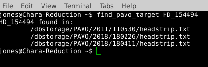
It is important that the HD number for the star be in the format HD_XXXXX, because the find_pavo_target script looks for the target in the same format as it appears in the headstrip file.

Setting up the PAVO environment

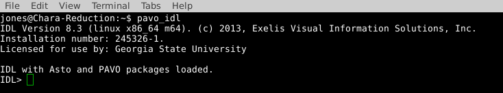
The PAVO data reduction software is written in IDL. The command pavo_idl will start IDL and load the astrolib IDL library and the PAVO software library. When you start IDL in this manner, you should see the following startup message:

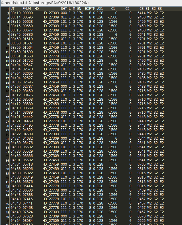
The headstrip.txt file

The first part of the data reduction process is to run the headstrip.pro program for the night of data you wish to reduce. We have already done this for all PAVO data currently in the archive, and we do this regularly as new PAVO data are copied to the archive. This program reads the header for each data file in the directory and outputs a text file in the data directory (headstrip.txt) containing the following information:

• UT – UT time of the first file
• FNUM – Starting file number
• HD – HD number of the Target
• SHT – Shutter status for beams B1, B2, and B3. “0” means open. “1” means closed. Taken as a whole, the three numbers indicate what part of the shutter sequence the data represent.
• GN – Gain setting of the detector
• EXPTM – Exposure time of the detector.
• C1, C2, C3 – Offsets for the OPLE carts. The carts are moved away from the fringe position during the shutters, so you should expect a different value in the shutter sequence compared to the data sequence.
• B1, B2, B3 – Identifies which telescope is on which beam

If you notice any discrepancies between your observing logs and the headstrip file, please discuss them with CHARA Data Scientist, Jeremy Jones before proceeding with your reduction as the headers on the data may need to be modified.

Tutorial Example - HD 154494

For this tutorial, we will reduce the data for one target and its two calibrators. These data were taken on UT 2018 Feb 26 with the S2-E2 baseline under decent seeing conditions (10.6 cm mean seeing for the night). Six observations were taken of the target, HD 154494, which is a V=4.8 magnitude star of type A3V with an estimated diameter of 0.38 mas (JMMC Stellar Diameter Catalogue). Four observations were taken of each calibrator. Both calibrators, HD 151862 and HD 154228, have V-band magnitudes of 5.9 mag and are A1V-type stars with estimated diameters of 0.22 mas.

Running processv2.pro

The first step of the reduction process that you will be running is processv2.pro. It can take several hours to run, so be prepared to wait. Processv2 requires the following to be set:

• Data directory – The name of the directory the data are in (not the full path). E.g., 180226
• The beams used – A vector of three integers of value 0 or 1 each representing which beams were used. E.g., [0,1,1] means beams 2 and 3 were used and [1,1,1] means all three beams were used.
• Starting file number – The number of the first file to be reduced. If you are reducing an entire night, this will be 00000 but you should consult the headstrip.txt file for your data if you are only reducing a portion of the night or if different configurations were used during the night.
• Ending file number – The number of the last file to be reduced.
• Output filename – The name you wish to give to the output file
• Root directory – The directory that the data directory is

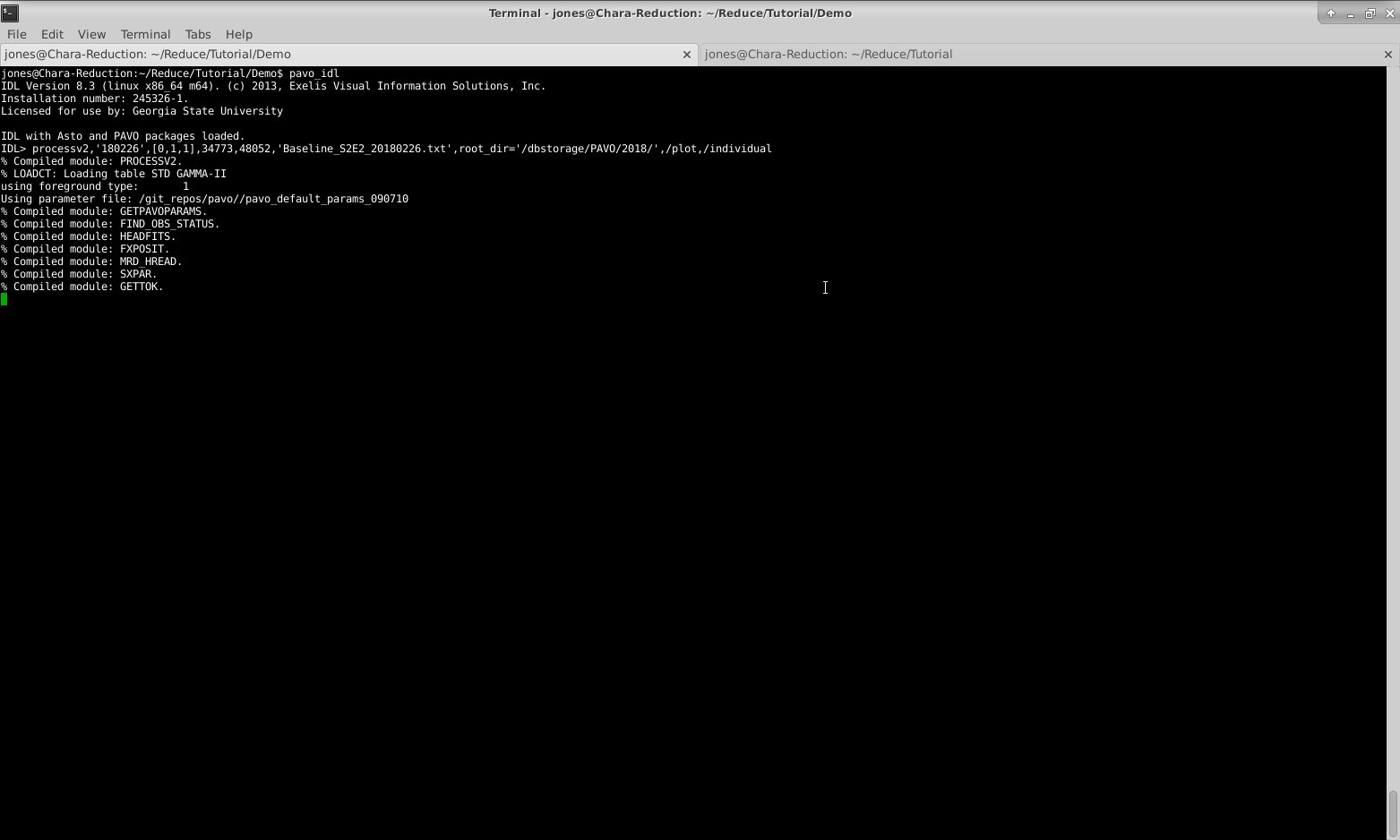
In our example, we will call the processv2 command like this:

processv2,’180226’,[0,1,1],34773,48052,’Baseline_S2E2_20180226.txt’,root_dir=’/dbstorage/PAVO/2018/’,/plot,/individual

In this case, 180226 is the data directory, [0,1,1] indicates we were using beams 2 and 3, 34773 is our starting file number, 48052 is our ending file number, Baseline_S2E2_20180226.txt is the name we’ve given to the output file, /dbstorage/PAVO/2018/ is the full path to the data directory, and the /plot and /individual flags are set (see below).

Note: You will need to run processv2 from your own working directory. If you try to run processv2 in the data directory, it will fail because you do not have permission to write in those directories. Options that can be set while running processv2 are:

• /nohann – Usually, a window is applied in the Fourier domain. Setting this keyword means that a window is not used.
• lambda_smooth=n – This option specifies the number of n wavelength channels over which signal will be coherently smoothed over to increase S/N by √ n . This can be used for data on faint stars but should be used with caution. In general, it is best to not set lambda_smooth for your first analysis and check the influence of lambda_smooth if you are not satisfied with the results.
• /individual – With this option set, processv2 will reduce all individual files. This is essential for rejecting bad data.
• /plot – This option displays plots during the reduction. Always use this option when you are running a new data analysis.

The outputs from processv2 are:

• Output file – A text file containing V2 values, estimated errors, closure phases, etc.
• The .pav file from individual analysis. These are IDL variable files that contain finely sampled V2 and closure-phase.
• The log file, which contains the settings used for the out file.
• If /plot is set, a screenshot of the output of the wavelength calibration will be created. A faulty wavelength calibration has strong potential to screw things up, and it should therefore be checked before proceeding in the analysis. Offsets and Rotation are listed in the log file: Offsets of +/- 2 pixels are ok, everything higher should be suspicious.

Starting processv2:

Wavelength calibration in processv2:

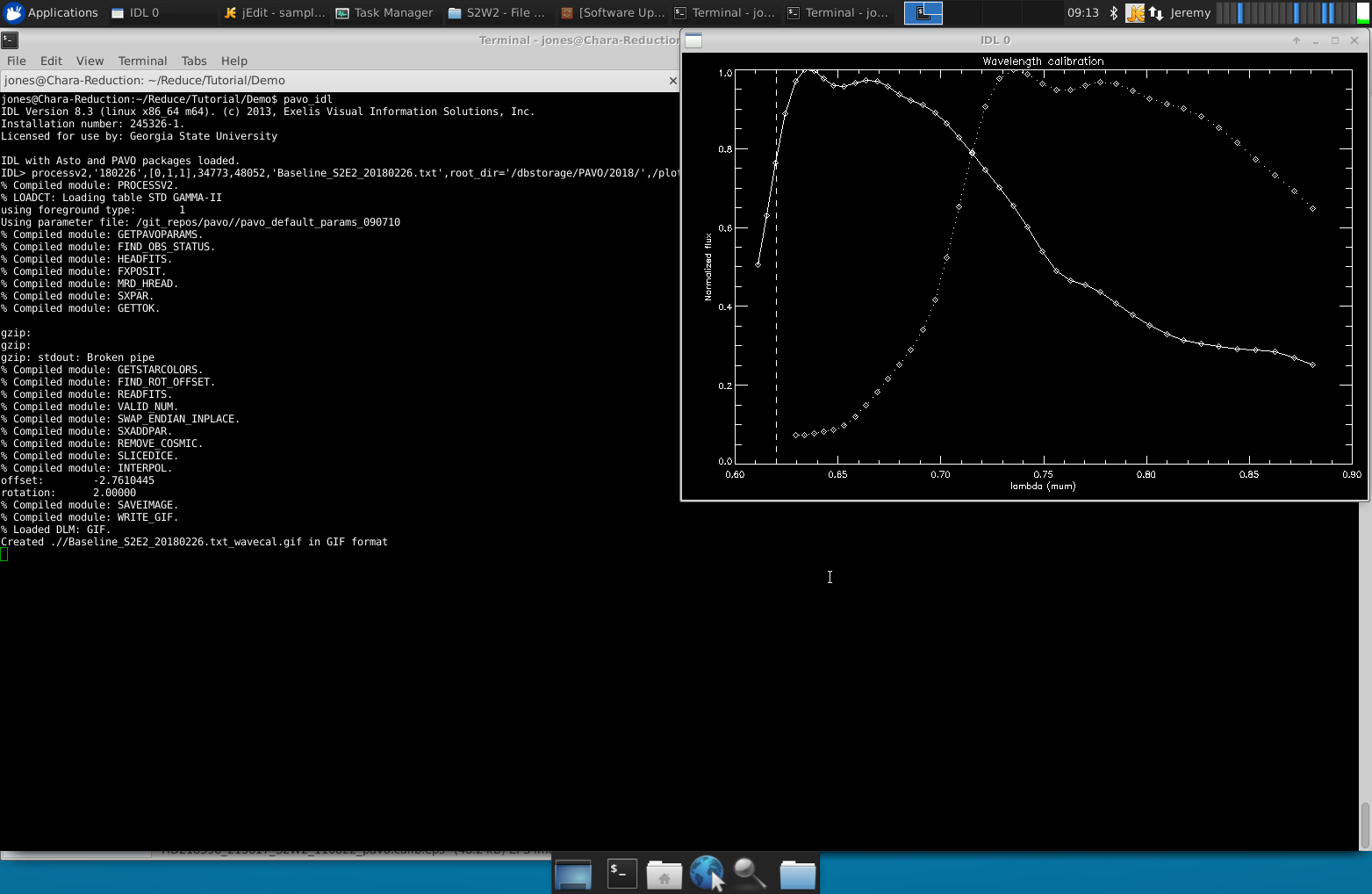
The solid line is flux vs. wavelength after correcting for offset. The dashed line is the calibrated inflection point of the PAVO filter. Example of the power spectra you should see during processv2:

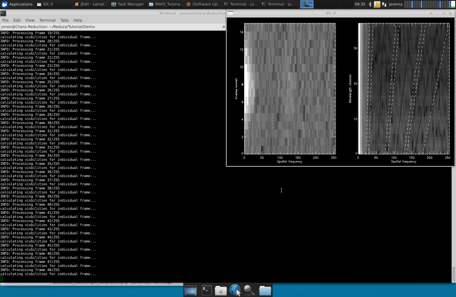
This is a good first quality test of your data. You should see a signal in these plots for your science data. Note: processv2 cannot process multiple baselines in one run. For example, if S2-E2 was used for the first half of the night and E2-W2 for the second half, processv2 cannot be run for the whole night. It should be run twice (once for the S2-E2 data and once for the E2-W2 data). Another option is to run processv2 separately for each target set (a target plus its calibrators) as we are doing in our example for HD 154494 and its calibrators.

Preparation for l0_l1_gui.pro

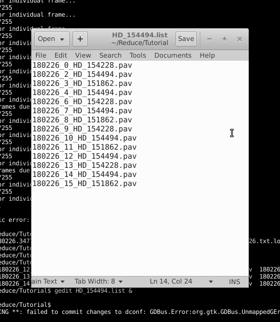
This program reduces level 0 data (the .pav files) to level 1 data (reduced, uncalibrated data). l0_l1_gui takes the .pav files and performs an automated outlier rejection as well as enables the user to manually reject bad sections of data. This program can only be run if /individual is set when running processv2. Create a text file that contains a list of the .pav files you will be reducing. To do this, exit the IDL environment and run the command ls *pav > yourlist.list. In our example, I have named the list file HD_154494.list. Because of how the ls function orders filenames, the items in your list may not be in chronological order. While l0_l1_gui.pro does not require the list to be in chronological order, you may find it easier if you reorder the list.

Running l0_l1_gui.pro

To start the GUI, enter the IDL environment with pavo_idl and start the GUI with l0_l1_gui.

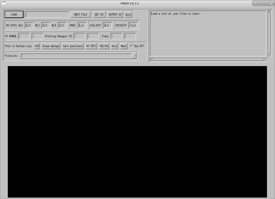
Click on the LOAD button to load yourlist.list. The output files for all scans will be called yourlist.list_l0_l1.res (or HD_154494.list_l0_l1.res for our example list).

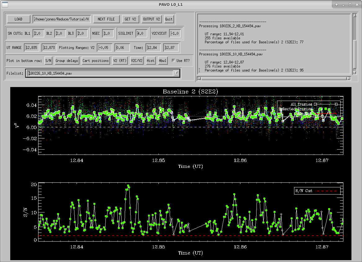
l0_l1_gui will start showing results for the first .pav file. The top panel displays UT time vs squared visibility. The bottom panel displays UT time vs. the signal to noise ratio. This S/N is calculated in real-time and is the value you see in the PAVO server during observing. In the top panel, each wavelength is shown as colored dots, and the white squares are the average V² over all wavelengths. Green squares are frames which are kept with the current rejection criteria. Outlier rejection is based on three criteria: S/N, seconds after the lock on the fringes is lost (NSEC), and deviation from the mean in sigma (SIGMA LIMIT). The default values should be fine in most cases. S/N cuts are the most appropriate to be adjusted if data is particularly bad or good. The window in the top right shows what percentage of recorded data files will be used for each baseline given the current rejection criteria. The plot on the bottom panel can be changed by clicking one of the options on the “Plot in bottom row” line. 

• S/N –This is the default secondary plot. It shows the UT time vs. the signal to noise ratio as well as a line showing where the S/N cut is currently set.
• Group delays – This shows the UT time vs. the group delay.
• Cart Positions – This shows the UT time vs. the position of the moving cart
• V2 (RT) – This shows the UT time vs. the squared visibilities calculated in real time during observing.
• V2C/V2 – This is an indirect measure of t₀ (good if high).
• Hist – This shows a histogram of how far each measured visibility point deviates from the mean visibility.
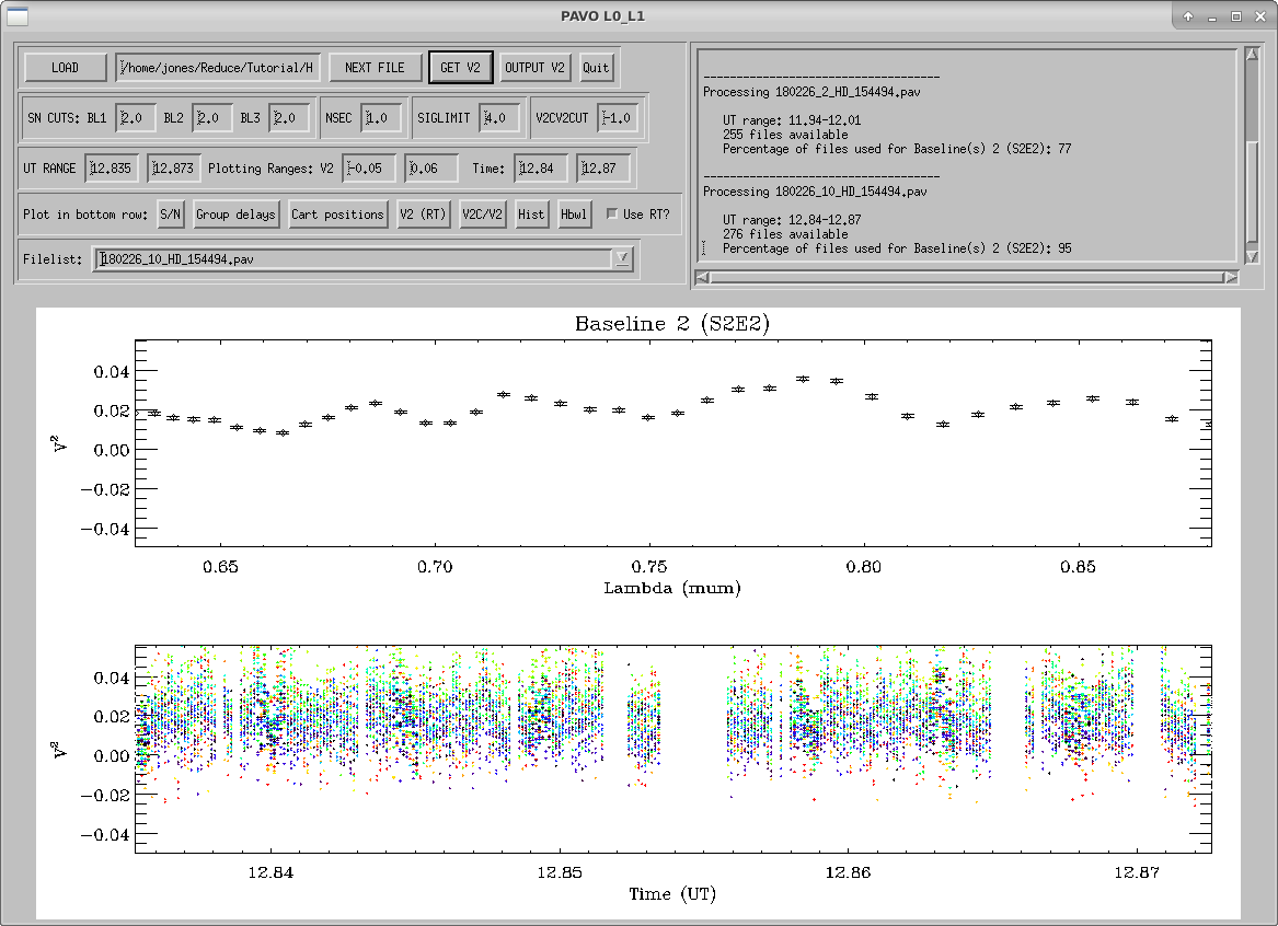
• Hbwl – This shows the same thing as the Hist option but broken up by wavelength channel. Once you’re satisfied with the rejection settings for the scan, press GET V2 to see the average squared visibilities that survived the outlier rejection plotted over wavelength (top plot) and the individual squared visibilities plotted over UT time with colors indicating different wavelength channels (bottom plot).

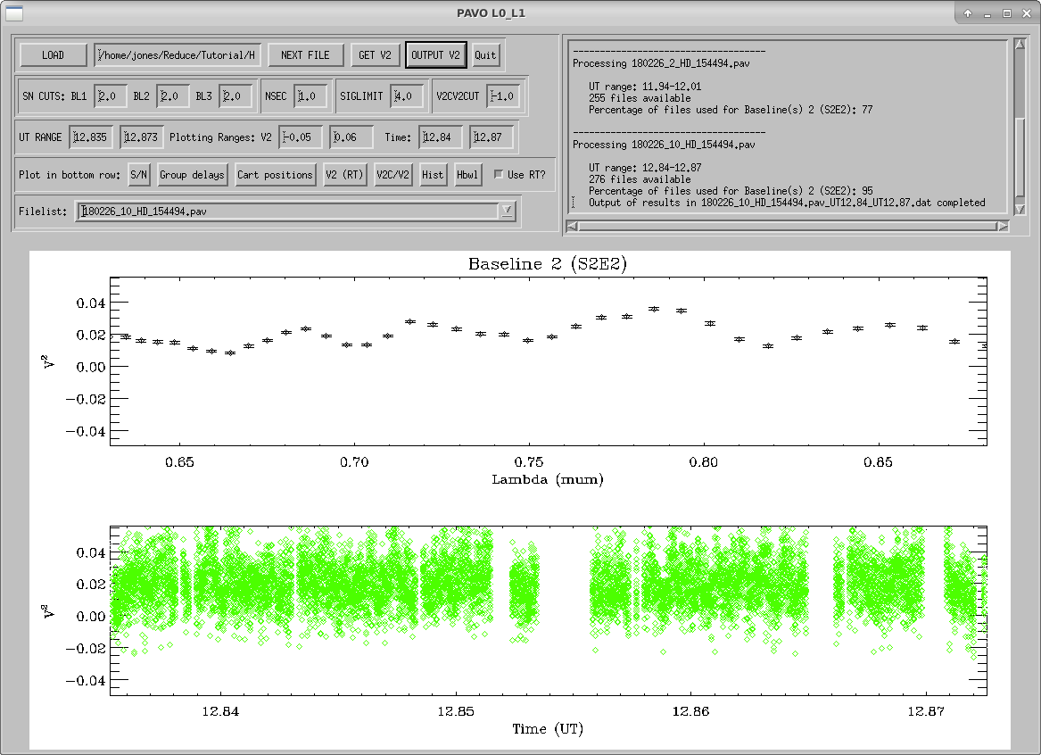
Then, press OUTPUT V2 to save your work. This will create an entry in the output file (yourlist.list_l0_l1.res) and some additional files that are used in the next step of the reduction.

Press NEXT FILE to start on the next .pav file and repeat the process with GET V2, OUTPUT V2, and NEXT FILE until all files have been reduced, at which point, the program will end. Note: If you are adjusting outlier rejection criteria, it is a good idea to use a single set of criteria for the entire night (rather than adjusting them star-by-star) in order to avoid bias in your calibration. Ideally, you shouldn’t have to adjust anything, and simply use the graphical inspection to decide which scans are useful for calibration and which are not.

Preparation for l1_l2_gui.pro

This program calibrates the level 1 visibility data that was reduced by l0_l1_gui.pro. This includes multi-bracket calibration and uncertainty calculations using Monte-Carlo simulations. Before running l1_l2_gui, you must create the following two files:

• A list of calibrators and their diameters
• A configuration file

Calibrator diameters

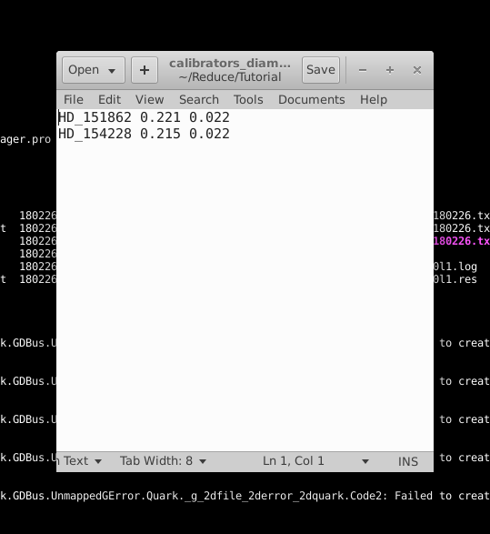
Create a text file with the calibrator’s name (in the same format as it shows up in the previous steps of the reduction process), its estimated angular diameter, and the uncertainty in this estimated angular diameter. In our example, this file is called calibrators_diam.dat.

Configuration file

Create a configuration file (in our example, this file is called HD_154494.config) in the following format:

; configuration file for multi-bracket diameter fitting using Monte-Carlo simulations ;;;;;;;;;;;;;;;;;;;;;;;;;;;;;;;;;;;;;;;;;;;;;;;;;;;;;;;;;;;;;;;;;;;;;;;;;;;;;;;;;;;;;;;;;;;
5041. ; number of MC iterations
1. ; lambda_smooth value used
0.4 ; initial guess for target diameter
0.628 ; linear limb darkening coefficent
0.02 ; absolute uncertainty on linear limb darkening coefficient
5. ; absolute uncertainty on wavelength scale (nm)
5. ; relative uncertainty on calibrator diameters (%)
;;;;;;;;;;;;;;;;;;;;;;;;;;;;;;;;;;;;;;;;;;;;;;;;;;;;;;;;;;;;;;;;;;;;;;;;;;;;;;;;;;;;;;;;;;;
;bracket 1 (first line: Target scans; second line: Calibrator Scans)
180226_2_HD_154494.pav
180226_0_HD_154228.pav,180226_3_HD_151862.pav
;bracket 2
180226_4_HD_154494.pav
180226_3_HD_151862.pav,180226_6_HD_154228.pav
;bracket 3
180226_7_HD_154494.pav
180226_6_HD_154228.pav,180226_8_HD_151862.pav
;bracket 4
180226_10_HD_154494.pav
180226_9_HD_154228.pav,180226_11_HD_151862.pav
;bracket 5
180226_12_HD_154494.pav
180226_11_HD_151862.pav,180226_13_HD_154228.pav
;bracket 6
180226_14_HD_154494.pav
180226_13_HD_154228.pav,180226_15_HD_151862.pav


Note: Two common scenarios that will cause l1_l2_gui to crash are:

• if the number of MC iterations is not a perfect square (the code expects the square root of this value to be an integer)
• if there is a blank line in the configuration file

Running l1_l2_gui.pro

To start the GUI, enter the IDL environment with pavo_idl and start the GUI with l1_l2_gui. Click INPUT FILE to select the results from l0_l1_gui (in our example, this is HD154494.list_l0l1.res). The first time you load this input file, l1_l2_gui will search for the stars’ coordinates using querysimbad to calculate projected baselines, which will take a few seconds per star. It will display this information in the window on the upper right of the GUI and it will save the information in an IDL savefile (in our example, this is called HD_154494.list_l0l1.res.idl) so you won’t have to wait as long when you load the results file in the future.

Click CAL DIAMETERS to load your calibrator diameters file.

Click LOAD CONFIG FILE to load your configuration file.

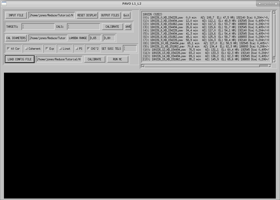
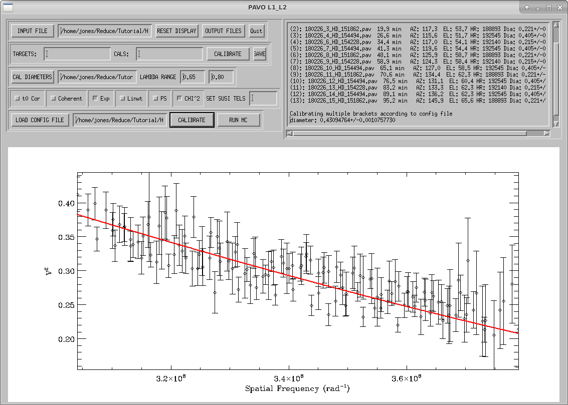
To calibrate your data in the manner listed in your configuration file, click the CALIBRATE button on the bottom row. If you wish to calibrate individual targets, you can input the target and calibrator indices in the TARGETS: and CALS: text boxes. These indices are the numbers in parentheses preceding the star information in the window in the upper right corner. This can be useful for identifying bad calibrators by calibrating them against each other. The following options can be set using either calibration method: 

• t0 Cor - Corrects for t₀
• Coherent - Uses the V²C values from l0_l1_gui instead of V²
• Exp - Uses the photometry to correct visibilities for photometric fluctuations.
• Linwt - Uses a linear weight rather than a quadratic weight for calculating weighted means in calibration.
• PS - Plots the Spatial Frequency vs. V² data so that the full visibility curve is seen (V² from 0 to 1 and Spatial Frequency from 0 to 5×10⁸ rad^-1)
• CHI^2 - Scales the reduced χ² such that the minimum reduced χ² is 1.
• SET SUSI TELS - This is used only for data taken from the beam combiner on the SUSI interferometer. The CALIBRATE button will also perform a least squares fit of a limb-darkened disk to the visibility curve.

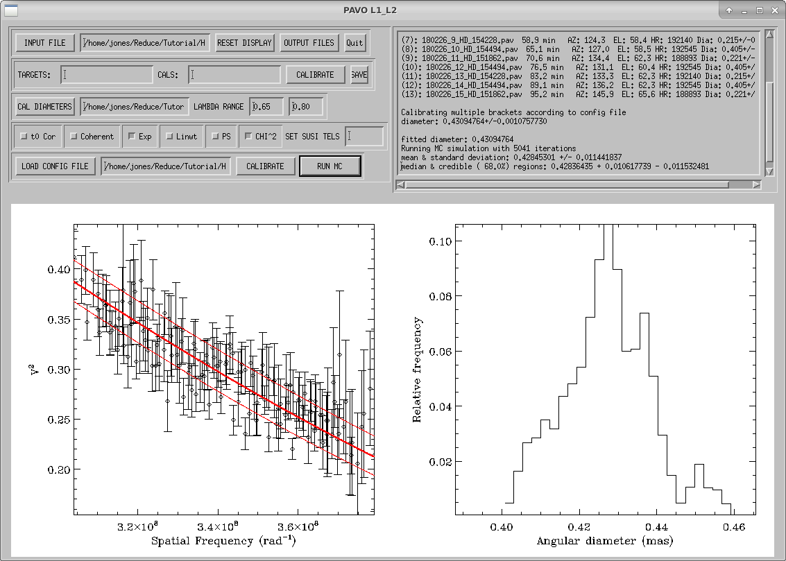
The RUN MC button will start Monte-Carlo simulations to calculate uncertainties in the limb-darkened diameter fit to the data. These simulations include uncertainties in the wavelength scale, calibrator diameters, measurement errors, limb-darkening coefficient, and correlations between wavelength channels.

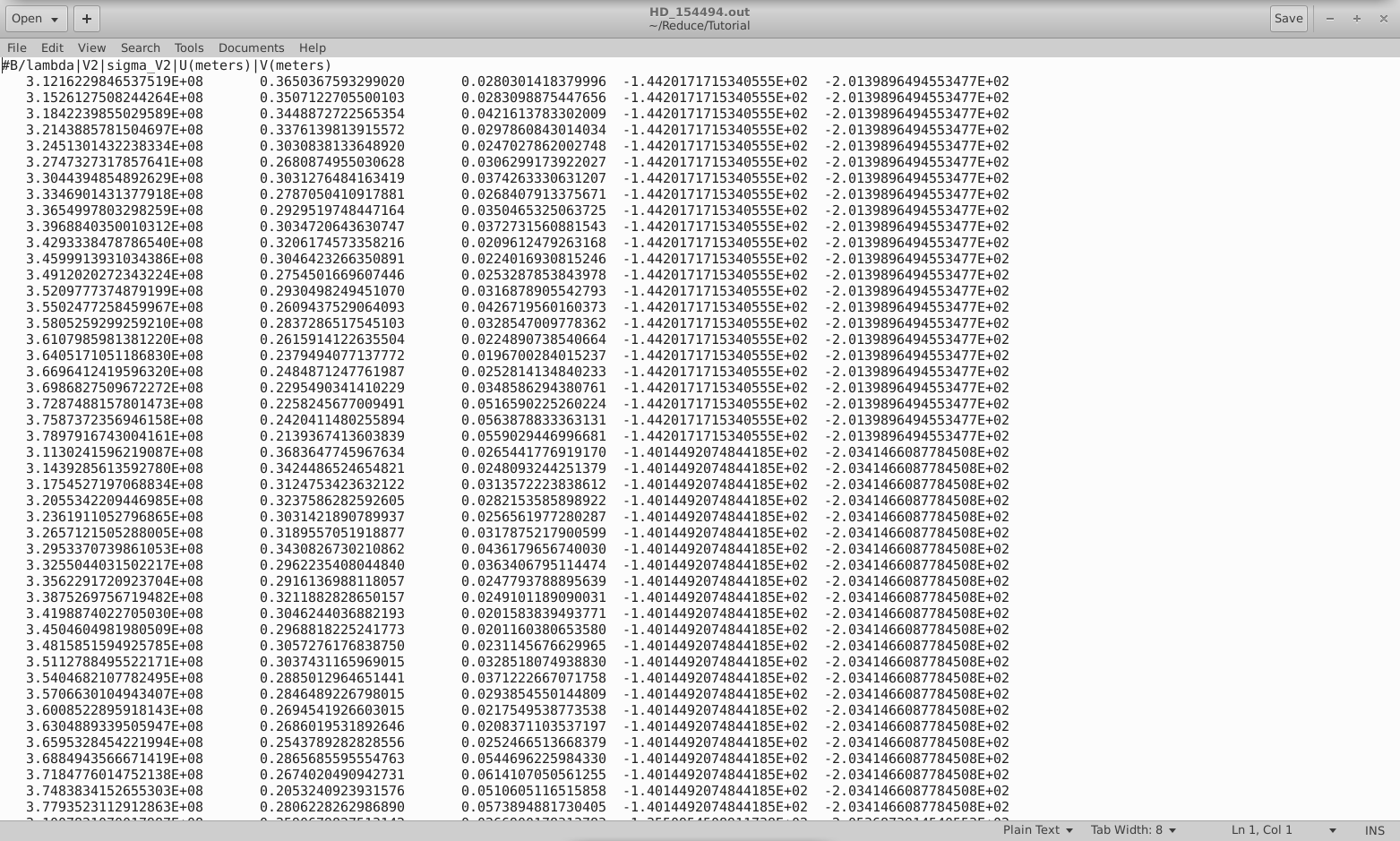
The OUTPUT FILES button will output your calibrated visibilities to a text file (in our case, I've named this file HD_154494.out). This text file saves the baseline divided by wavelength, squared visibility, uncertainty in the squared visibility, and U- and V- coordinates for each calibrated visibility measurement.

Converting Results to the OIFITS format

The python script, pavo2T_to_oifits.py (written by Guillaume Schworer) converts the output files of l1_l2_gui into OIFITS format. You can call this script by running the command pavo2T_to_oifits.py <Input Directory> <l0_l1_gui Input Filename> <Output Directory (optional)>

. In our example, we would call pavo2T_to_oifits.py "/home/jones/Reduce/Tutorial/" "HD_154494.list". If the output directory is not given, the output oifits file (in our case, called HD_154494.list.oifits) will be put in the input directory.